2.4.6: Examples of Derivations

\(\def\Assign#1#2{ { #1^{\Struct{#2}} } }\)
\(\def\Atom#1#2{ { \mathord{#1}(#2) } }\)
\(\def\Bin{ {\mathbb{B}} }\)
\(\def\cardeq#1#2{ { #1 \approx #2 } }\)
\(\def\cardle#1#2{ { #1 \preceq #2 } }\)
\(\def\cardless#1#2{ { #1 \prec #2 } }\)
\(\def\cardneq#1#2{ { #1 \not\approx #2 } }\)
\(\def\comp#1#2{ { #2 \circ #1 } }\)
\(\def\concat{ { \;\frown\; } }\)
\(\def\Cut{ { \text{Cut} } }\)
\(\def\Discharge#1#2{ { [#1]^#2 } }\)
\(\def\DischargeRule#1#2{ { \RightLabel{#1}\LeftLabel{\scriptsize{#2} } } }\)
\(\def\dom#1{ {\operatorname{dom}(#1)} }\)
\(\def\Domain#1{ {\left| \Struct{#1} \right|} }\)
\(\def\Elim#1{ { {#1}\mathrm{Elim} } }\)
\(\newcommand{\Entails}{\vDash}\)
\(\newcommand{\EntailsN}{\nvDash}\)
\(\def\eq[#1][#2]{ { #1 = #2 } }\)
\(\def\eqN[#1][#2]{ { #1 \neq #2 } }\)
\(\def\equivclass#1#2{ { #1/_{#2} } }\)
\(\def\equivrep#1#2{ { [#1]_{#2} } }\)
\(\def\Exchange{ { \text{X} } }\)
\(\def\False{ { \mathbb{F} } }\)
\(\def\FalseCl{ { \lfalse_C } }\)
\(\def\FalseInt{ { \lfalse_I } }\)
\(\def\fCenter{ { \,\Sequent\, } }\)
\(\def\fdefined{ { \;\downarrow } }\)
\(\def\fn#1{ { \operatorname{#1} } }\)
\(\def\Frm[#1]{ {\operatorname{Frm}(\Lang #1)} }\)
\(\def\fundefined{ { \;\uparrow } }\)
\(\def\funimage#1#2{ { #1[#2] } }\)
\(\def\funrestrictionto#1#2{ { #1 \restriction_{#2} } }\)
\(\newcommand{\ident}{\equiv}\)
\(\newcommand{\indcase}[2]{#1 \ident #2\text{:}}\)
\(\newcommand{\indcaseA}[2]{#1 \text{ is atomic:}}\)
\(\def\indfrm{ { A } }\)
\(\def\indfrmp{ { A } }\)
\(\def\joinrel{\mathrel{\mkern-3mu}}\)
\(\def\lambd[#1][#2]{\lambda #1 . #2}\)
\(\def\Lang#1{ { \mathcal{#1} } }\)
\(\def\LeftR#1{ { {#1}\mathrm{L} } }\)
\(\def\len#1{ {\operatorname{len}(#1)} }\)
\(\def\lexists#1#2{ { \exists #1\, #2 } }\)
\(\def\lfalse{ {\bot} }\)
\(\def\lforall#1#2{ { \forall#1\, #2 } }\)
\(\newcommand{\lif}{\rightarrow}\)
\(\newcommand{\liff}{\leftrightarrow}\)
\(\def\Log#1{ { \mathbf{#1} } }\)
\(\def\ltrue{ {\top} }\)
\(\def\Id#1{ {\operatorname{Id}_#1} }\)
\(\def\Int{ {\mathbb{Z}} }\)
\(\def\Intro#1{ { {#1}\mathrm{Intro} } }\)
\(\def\mModel#1{ { \mathfrak{#1} } }\)
\(\newcommand{\mSat}[3][{}]{\mModel{#2}{#1}\Vdash{#3}}\)
\(\newcommand{\mSatN}[3][{}]{\mModel{#2}{#1}\nVdash{#3}}\)
\(\def\Nat{ {\mathbb{N}} }\)
\(\def\nicefrac#1#2{ {{}^#1/_#2} }\)
\(\def\num#1{ { \overline{#1} } }\)

\(\def\ran#1{ {\operatorname{ran}(#1)} }\)
\(\newcommand{\Obj}[1]{\mathsf{#1}}\)
\(\def\Rat{ {\mathbb{Q}} }\)
\(\def\Real{ {\mathbb{R}} }\)
\(\def\RightR#1{ { {#1}\mathrm{R} } }\)
\(\def\Part#1#2{ { \Atom{\Obj P}{#1, #2} } }\)
\(\def\pto{ { \hspace{0.1 cm}\to\hspace{-0.44 cm}\vcenter{\tiny{\hbox{|}}}\hspace{0.35 cm} } }\)
\(\def\PosInt{ {\mathbb{Z}^+} }\)
\(\def\Pow#1{ {\wp(#1)} }\)
\(\newcommand{\Proves}{\vdash}\)
\(\newcommand{\ProvesN}{\nvdash}\)
\(\def\Relbar{\mathrel{=}}\)
\(\newcommand{\Sat}[3][{}]{\Struct{#2}{#1}\vDash{#3}}\)
\(\newcommand{\SatN}[3][{}]{\Struct{#2}{#1}\nvDash{#3}}\)
\(\newcommand{\Sequent}{\Rightarrow}\)
\(\def\Setabs#1#2{ { \{#1:#2\} } }\)
\(\newcommand{\sFmla}[2]{#1\,#2}\)
\(\def\Struct#1{ {#1} }\)
\(\def\subst#1#2{ { #1/#2 } }\)
\(\def\Subst#1#2#3{ { #1[\subst{#2}{#3}] } }\)
\(\def\TMblank{ { 0 } }\)
\(\newcommand{\TMendtape}{\triangleright}\)
\(\def\TMleft{ { L } }\)
\(\def\TMright{ { R } }\)
\(\def\TMstay{ { N } }\)
\(\def\TMstroke{ { 1 } }\)
\(\def\TMtrans#1#2#3{ { #1,#2,#3 } }\)
\(\def\Trm[#1]{ {\operatorname{Trm}(\Lang #1)} }\)
\(\def\True{ { \mathbb{T} } }\)
\(\newcommand{\TRule}[2]{#2#1}\)
\(\def\tuple#1{ {\langle #1 \rangle} }\)
\(\newcommand{\Value}[3][\,]{\mathrm{Val}_{#1}^{#3}(#2)}\)
\(\def\Var{ { \mathrm{Var} } }\)
\(\newcommand{\varAssign}[3]{#1 \sim_{#3} #2}\)
\(\def\Weakening{ { \text{W} } }\)

Example \(\PageIndex{1}\)

Give an \(\Log{LK}\)-derivation for the sequent \(A \land B \Sequent A\).

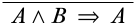
We begin by writing the desired end-sequent at the bottom of the derivation.

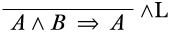
Next, we need to figure out what kind of inference could have a lower sequent of this form. This could be a structural rule, but it is a good idea to start by looking for a logical rule. The only logical connective occurring in the lower sequent is \(\land\), so we’re looking for an \(\land\) rule, and since the \(\land\) symbol occurs in the antecedent, we’re looking at the \(\LeftR{\land}\) rule.

There are two options for what could have been the upper sequent of the \(\LeftR{\land}\) inference: we could have an upper sequent of \(A \Sequent A\), or of \(B \Sequent A\). Clearly, \(A \Sequent A\) is an initial sequent (which is a good thing), while \(B \Sequent A\) is not derivable in general. We fill in the upper sequent:

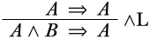
We now have a correct \(\Log{LK}\)-derivation of the sequent \(A \land B \Sequent A\).

Example \(\PageIndex{2}\)

Give an \(\Log{LK}\)-derivation for the sequent \(\lnot A \lor B \Sequent A \lif B\).

Begin by writing the desired end-sequent at the bottom of the derivation.

To find a logical rule that could give us this end-sequent, we look at the logical connectives in the end-sequent: \(\lnot\), \(\lor\), and \(\lif\). We only care at the moment about \(\lor\) and \(\lif\) because they are main operators of sentences in the end-sequent, while \(\lnot\) is inside the scope of another connective, so we will take care of it later. Our options for logical rules for the final inference are therefore the \(\LeftR{\lor}\) rule and the \(\RightR{\lif}\) rule. We could pick either rule, really, but let’s pick the \(\RightR{\lif}\) rule (if for no reason other than it allows us to put off splitting into two branches). According to the form of \(\RightR{\lif}\) inferences which can yield the lower sequent, this must look like:

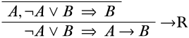
If we move \(\lnot A \lor B\) to the outside of the antecedent, we can apply the \(\LeftR{\lor}\) rule. According to the schema, this must split into two upper sequents as follows:

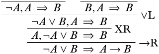
Remember that we are trying to wind our way up to initial sequents; we seem to be pretty close! The right branch is just one weakening and one exchange away from an initial sequent and then it is done:

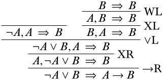
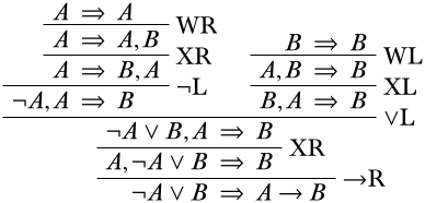
Now looking at the left branch, the only logical connective in any sentence is the \(\lnot\) symbol in the antecedent sentences, so we’re looking at an instance of the \(\LeftR{\lnot}\) rule.

Similarly to how we finished off the right branch, we are just one weakening and one exchange away from finishing off this left branch as well.

Example \(\PageIndex{3}\)

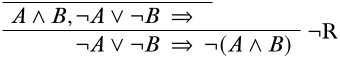
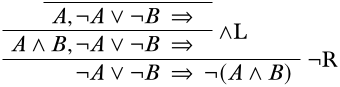
Give an \(\Log{LK}\)-derivation of the sequent \(\lnot A \lor \lnot B \Sequent \lnot (A \land B)\)

Using the techniques from above, we start by writing the desired end-sequent at the bottom.

The available main connectives of sentences in the end-sequent are the \(\lor\) symbol and the \(\lnot\) symbol. It would work to apply either the \(\LeftR{\lor}\) or the \(\RightR{\lnot}\) rule here, but we start with the \(\RightR{\lnot}\) rule because it avoids splitting up into two branches for a moment:

Now we have a choice of whether to look at the \(\LeftR{\land}\) or the \(\LeftR{\lor}\) rule. Let’s see what happens when we apply the \(\LeftR{\land}\) rule: we have a choice to start with either the sequent \(A, \lnot A \lor B \Sequent \quad\) or the sequent \(B, \lnot A \lor B \Sequent \quad\). Since the proof is symmetric with regards to \(A\) and \(B\), let’s go with the former:

Continuing to fill in the derivation, we see that we run into a problem:

The top of the right branch cannot be reduced any further, and it cannot be brought by way of structural inferences to an initial sequent, so this is not the right path to take. So clearly, it was a mistake to apply the \(\LeftR{\land}\) rule above. Going back to what we had before and carrying out the \(\LeftR{\lor}\) rule instead, we get

Completing each branch as we’ve done before, we get

(We could have carried out the \(\land\) rules lower than the \(\lnot\) rules in these steps and still obtained a correct derivation).

Example \(\PageIndex{4}\)

So far we haven’t used the contraction rule, but it is sometimes required. Here’s an example where that happens. Suppose we want to prove \(\quad \Sequent A \lor \lnot A\). Applying \(\RightR{\lor}\) backwards would give us one of these two derivations:

Neither of these of course ends in an initial sequent. The trick is to realize that the contraction rule allows us to combine two copies of a sentence into one—and when we’re searching for a proof, i.e., going from bottom to top, we can keep a copy of \(A \lor \lnot A\) in the premise, e.g.,

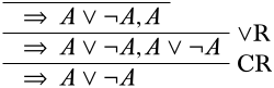
Now we can apply \(\RightR{\lor}\) a second time, and also get \(\lnot A\), which leads to a complete derivation.

Problem \(\PageIndex{1}\)

Give derivations of the following sequents:

1. \(\Sequent \lnot(A \lif B) \lif (A \land \lnot B)\)
2. \((A \land B) \lif C \Sequent (A \lif C) \lor (B \lif C)\)