7.5: Logical Analysis using Truth Tables

Truth tables, which we introduced in the last section, are primarily useful in a different way. Instead of just using them to tell us what the different logical operators mean, we can use them to do some in depth analysis of the logical form of a statement, a set of statements, or an inference.

What’s a logical analysis? A logical analysis is a set of things we can do to learn something about a particular logical structure. The statement “I’ll go if you don’t go or if we can get a babysitter and it’s not too expensive for both of us to go” has a particular logical form—something like

[(B\(\wedge\)~E)\(\rightarrow\)I]. If we do a logical analysis of this logical form, we’ll find out certain things. For instance: when is this statement true? That is, what must the world be like for this statement to turn out to be true? Is this statement always true? Is it always false? What is its relationship with other similar logical forms like [~(B\(\wedge\)E)\(\rightarrow\)I]? [~(B\(\wedge\)~E)\(\rightarrow\)~I]? [(B\(\wedge\)E)\(\rightarrow\)~I]? Is it possible that all of these statements could be true at the same time? That is, are they consistent? We can find out the answers to all of these questions using Truth Tables.

Conceptually speaking, we’re doing the following when we build a truth table:

1. Collecting all of the possible combinations of truth values and listing them out.

• That is, we’re finding out all of the different ways that T and F can be combined for our atomic sentence letters.

2. Using each set of possible truth values to calculate the output truth value for a complex formula (or a set of complex formulas).

• That is, we’re doing what we did in Computing Truth Values: we’re taking the truth values of atomic sentence letters as an input and calculating the single truth value output.

3. Analyzing the results.

• That is, we’re looking at the resulting output and trying to figure out what it tells us about the logical formulas in question.

The goal is to see what possible conditions of the world (what combinations of true and false for the atomic propositions, each of which either describes the world correctly or incorrectly) give what sorts of truth values for the complex formulas we’re analyzing and then to look for patterns in the outputs to tell us something about the individual statement, the set of statements, or the argument we’re analyzing.

That’s not terribly illuminating, though, about how to actually go about building a truth table. Let’s look more concretely at what to do.

First, I must point out a new notation that will be unfamiliar to you. Well, you will have seen it before lots of times, but not here in logic. The forward slash!

If you see this:

[\(\neg\)[D \(\leftrightarrow\) \(\neg\)(X\(\rightarrow\) (Z \(\bullet\) Q))] \(\vee\) P] / (X\(\rightarrow\) (Z \(\bullet\) Q))]

That means there are two formulas here:

[\(\neg\)[D \(\leftrightarrow\) \(\neg\)(X\(\rightarrow\) (Z \(\bullet\) Q))] \(\vee\) P]

And

(X\(\rightarrow\) (Z \(\bullet\) Q))]

The forward slash (/) has no logical meaning. It simply separates formulas from one another so we can list them on a single line without it seeming like they are parts of the same formula.

Building a Truth Table

Building a truth table is very straightforward, but that doesn’t mean it’s not going to take some getting used to. Let’s divide it into a series of steps.

Step One: Figure out what size you need

How many unique sentence letters are in the formula or set of formulas? Just count ‘em up, counting each unique letter only once (so two B’s just count as one). Here are some examples:

• [~(B\(\wedge\)E)\(\rightarrow\)I] has 3 unique letters: B, E, and I
• [~(B\(\wedge\)E)\(\rightarrow\)B] has 2 unique letter: B and E
• [~(I\(\wedge\)I)\(\rightarrow\)I] has 1 unique letter: I
• [~(B\(\wedge\)E)\(\rightarrow\)I] / [(B\(\wedge\)E)\(\rightarrow\)~I] have 3 unique letters all together: B, E, and I
• [\(\neg\)[D \(\leftrightarrow\) \(\neg\)(X\(\rightarrow\) (Z \(\bullet\) Q))] \(\vee\) P] / Z / (P \(\bullet\) Q) has 5 unique letters: D, X, Z, Q, and P

Once you’ve figure out this magic number, you plug it into a magic formula: 2ⁿ, where n is the magic number: the number of unique sentence letters in the set of propositions the truth table is for. The result of this mathematical formula is the number of rows you’ll need in your truth table.

Here are a set of truth table sizes:

# of unique letters	# of rows
1	2
2	4
3	8
4	16
5	32
6	64
16	65,536

Notice the pattern? The nice thing is that chances are, your instructor will only assign at most a 4-letter truth table, so 16 rows is the absolute most you’ll usually need to work with. Most instructors stick to 1, 2, and 3-letter truth tables.

The downside of truth tables is that it doesn’t take long before you have to start making tables with 32, 64, 128, 256, 512, 65,536 rows! That’s too much to really make making a truth table worthwhile. This is called the problem of Combinatorial Explosion because all of the combinations that are possible “explode” to astronomical numbers. Nevertheless, they are quite useful for relatively simple problems.

Step Two: Make a truth table

A truth table is a table with a column for each unique sentence letter (usually in the order in which they show up in the formulas you are analyzing) and then a column for each formula you are analyzing. Here are some examples:

R	R\(\equiv\)(R\(\rightarrow\)R)	R\(\bullet\)\(\neg\)R

Q	R	R\(\equiv\)(Q\(\rightarrow\)R)	R\(\bullet\)\(\neg\)Q

Notice how each column gets its own label and there’s a bigger border separating the individual sentence letters (the inputs) from the complex formulas (the outputs). So far so good.

Step Three: Fill in the input side

This step is always the same no matter what the columns labels are. There are basically 3 different tables you’ll make, and for bigger tables you can extrapolate the same basic pattern. Remember that the goal when filling in the input side is to make a list of all of the possible combinations of the two truth values T and F.

So when we only have one unique sentence letter. The two possibilities are that the letter is True and the letter is False:

R	R \(\equiv\)(R\(\rightarrow\)R)	R\(\bullet\)\(\neg\)R
T
F

It’s a bit more complicated if we have two unique sentence letters:

Q	R	R\(\equiv\)(Q\(\rightarrow\)R)	R\(\bullet\)\(\neg\)Q
T	T
T	F
F	T
F	F

Each row in the table is a possible set of truth values. The possible combos are TT, TF, FT, and FF. See how that works?

Before moving onto an eight row truth table, let’s think about the pattern here. We’ve started on the right nearest the thick line separating the inputs from the outputs and alternated going down: TFTF. For the first table, we alternated too, but just had to do it once: TF. On the second table, we alternated TF going down the R column, and then just repeated so the downward pattern would be TFTF.

Then we moved left and alternated every 2, so the Q column reads TTFF. Why would we do this? Well, we have R is true and R is false, then we need to test for when Q is True with both of these possibilities, and then test again for when Q is false. The result is something like the following:

Q is True	R is True
	R is False
Q is False	R is True
	R is False

It may even be helpful to think of it in these terms:

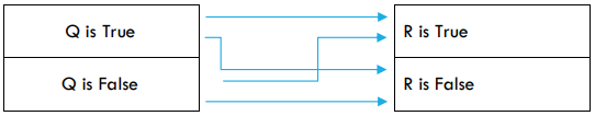
This way, we’re getting all the possible combinations of Q:true, Q:false, R:true, and R:false. If this little explanation is confusing for you, it’s probably best to move on. Perhaps it will make more sense later, and even if it doesn’t, it’s okay since this is sort of conceptual background work rather than something that is vital to understanding the truth table. What you need to understand at minimum is simply that by following this procedure, you’re creating all of the possible combinations of T and F for the atomic sentence letters in the formulas you are trying to analyze using the truth table.

Now let’s look at an eight row table. The first thing we do is start on the rightmost input (sentence letter) column, and alternate T and F every one row. Like so:

P	Q	R	P\(\equiv\)(Q\(\rightarrow\)R)	R\(\bullet\)\(\neg\)Q
		T
		F
		T
		F
		T
		F
		T
		F

Then we move one column to the left and alternate every two. Like this:

P	Q	R	P\(\equiv\)(Q\(\rightarrow\)R)	R\(\bullet\)\(\neg\)Q
	T	T
	T	F
	F	T
	F	F
	T	T
	T	F
	F	T
	F	F

Finally, we move to the left again and alternate every four rows so that we double the amount we are alternating by each time we move to the left. Like this:

P	Q	R	P\(\equiv\)(Q\(\rightarrow\)R)	R\(\bullet\)\(\neg\)Q
T	T	T
T	T	F
T	F	T
T	F	F
F	T	T
F	T	F
F	F	T
F	F	F

The result is a truth table that’s totally ready to solve: we have our columns labeled, our rows easily distinguishable, and most importantly we have all of the input side filled in in the standard way. This input side will be basically the same for every truth table. That is, you always follow this pattern:

Start below the rightmost atomic sentence letter and alternate every one row. Then move to the left one column and alternate going down every two rows. Finally, move to the left one last column and alternate going down that column every four rows. Extrapolate for bigger tables.

Solving a Truth Table

There are two methods to solving a truth table—filling in the right side or output side of the truth table. On the Brute Force method, you simply calculate each cell in the table by plugging the truth values of the sentence letters and working your way from the inside out. On the Intuitive method, you use your intuitive understanding of the operators to save yourself some work.

Brute Force Method

The Brute Force method to solving a truth table is simply to plug in the truth value for each individual letter by carrying them over from the input side and then calculating the truth value of each complex proposition given the truth values of the input side. This method is safer, so if you feel lost or lose confidence, then just revert back to the brute force method. It does have two downsides, though: a) It requires a lot more work and so takes more time, and b) it involves more individual steps and so the probably of making a simple mistake increases a bit. The second problem is probably balanced out by the riskiness of the Intuitive Method.

Write the truth value of each *letter* as it appears on the left side of the table under each letter as it appears on the right side

1. Starting with the “inner most” operators (inside the most parentheses) calculate the truth value of the whole relationship.

2. Then work your way out until you’ve calculated the truth value of the main operator.

So, step 0 is to make the truth table, as discussed in Basic Symbolization:

P	Q	(P \(\rightarrow\) (Q\(\leftrightarrow\)P))	(Q \(\leftrightarrow\) \(\neg\)(P\(\vee\)Q))
T	T
T	F
F	T
F	F

Step 1 is to fill in the truth values on the right side for the sentence letters

P	Q	(P \(\rightarrow\) (Q\(\leftrightarrow\)P))	(Q \(\leftrightarrow\) \(\neg\)(P\(\vee\)Q))
F	T	T T T	T T T
F	F
T	T
T	F

Step 2 is to find the inner most operators (the ones with the most amount of parentheses outside of them.

P	Q	(P \(\rightarrow\) \(\require{enclose} \enclose{circle}{(Q\leftrightarrow P)}\))	(Q \(\leftrightarrow\) \(\neg\)\(\enclose{circle}{(P\vee Q)}\))
F	T	T T T	T T T
F	F
T	T
T	F

And then solve for those values using the truth tables that we use to define each operator.

P	Q	(P \(\rightarrow\) (Q\(\leftrightarrow\)P))	(Q \(\leftrightarrow\) \(\neg\)(P\(\vee\)Q))
T	T	T T	T T
T	F
F	T
F	F

Repeat the steps in 2 (working from “in” to “out”) until you’ve solved the truth value of the main operators (the operators that are only inside the outermost parentheses. Keep in mind that if there are no outermost parentheses, then they are implied).

So Q \(\leftrightarrow\) (P\(\vee\)Q) is actually supposed to read: (Q \(\leftrightarrow\) (P\(\vee\)Q))

P	Q	(P \(\rightarrow\) (Q\(\leftrightarrow\)P))	(Q \(\leftrightarrow\) \(\neg\)(P\(\vee\)Q))
T	T	T T	T F
T	F
F	T
F	F

P	Q	(P \(\rightarrow\) (Q\(\leftrightarrow\)P))	(Q \(\leftrightarrow\) \(\neg\)(P\(\vee\)Q))
T	T	T	F
T	F
F	T
F	F

Repeat in each row:

P	Q	(P \(\rightarrow\) (Q\(\leftrightarrow\)P))	(Q \(\leftrightarrow\) \(\neg\)(P\(\vee\)Q))
T	T	\(\downarrow\) T \(\downarrow\) \(\downarrow\)	\(\downarrow\) F \(\downarrow\) \(\downarrow\)
T	F	T F T	F T F
F	T	F T F	T F T
F	F	F F F	F F F

P	Q	(P \(\rightarrow\) (Q\(\leftrightarrow\)P))	(Q \(\leftrightarrow\) \(\neg\)(P\(\vee\)Q))
T	T	\(\downarrow\) T \(\downarrow\)	\(\downarrow\) F \(\downarrow\)
T	F	T F	F T
F	T	F F	T T
F	F	F T	F F

P	Q	(P \(\rightarrow\) (Q\(\leftrightarrow\)P))	(Q \(\leftrightarrow\) \(\neg\)(P\(\vee\)Q))
T	T	\(\downarrow\) T \(\downarrow\)	\(\downarrow\) F \(\downarrow\)
T	F	T F	F F
F	T	F F	T F
F	F	F T	F T

P	Q	(P \(\rightarrow\) (Q\(\leftrightarrow\)P))	(Q \(\leftrightarrow\) \(\neg\)(P\(\vee\)Q))
T	T	T	F
T	F	F	T
F	T	T	F
F	F	T	F

Then you analyze the results by looking at the right side of the truth table!

P	Q	(P \(\rightarrow\) (Q\(\leftrightarrow\)P))	(Q \(\leftrightarrow\) \(\neg\)(P\(\vee\)Q))
T	T	T	F
T	F	F	T
F	T	T	F
F	F	T	F

Intuitive Method

The Intuitive Method to solving a truth table uses our intuitive understanding of the logical operators and their individual truth tables to save as much work as possible. We can often eliminate half of our work for one column in a single swoop.

It is a faster method, but also increases the chances that we’ll make a mistake by moving too quickly and missing something or being overconfident and ignoring important details.

How does it work? Let’s start with an example and then we’ll look at how it works a bit more.

P	Q	(P \(\rightarrow\) (Q\(\leftrightarrow\)P))	(Q \(\wedge\) \(\neg\)(P\(\vee\)Q))	(Q \(\wedge\) \(\neg\)P)
T	T
T	F
F	T
F	F

Starting with the first column, we ask ourselves what we know about the main operator (\(\rightarrow\)). I notice that there is only one atomic letter as the antecedent to this conditional. I know that if the antecedent to a conditional is false the whole conditional is true (since it’s only false when T\(\rightarrow\)F and if it’s F\(\rightarrow\)?, then it’s certainly not T\(\rightarrow\)F!). So I just need to find the rows on which P is false and I know the whole first formula will be True!

P	Q	(P \(\rightarrow\) (Q\(\leftrightarrow\)P))	(Q \(\wedge\) \(\neg\)(P\(\vee\)Q))	(Q \(\wedge\) \(\neg\)P)
T	T
T	F
F	T	T
F	F	T

Then we solve the rest more-or-less using the Brute Force method. When is (Q\(\leftrightarrow\)P) true? When they’re the same! It’s false if they’re different.

P	Q	(P \(\rightarrow\) (Q\(\leftrightarrow\)P))	(Q \(\wedge\) \(\neg\)(P\(\vee\)Q))	(Q \(\wedge\) \(\neg\)P)
T	T	T
T	F	F
F	T	T
F	F	T

Now we look at the second column. When is a conjunction true? It’s only true in one case: when both conjuncts are true. So if Q is false...? Then the whole second formula (Q \(\wedge\) \(\neg\)(P\(\vee\)Q)) is false.

P	Q	(P \(\rightarrow\) (Q\(\leftrightarrow\)P))	(Q \(\wedge\) \(\neg\)(P\(\vee\)Q))	(Q \(\wedge\) \(\neg\)P)
T	T	T
T	F	F	F
F	T	T
F	F	T	F

Now that we know Q is true in the remaining cells of the second output column, we need to ask ourselves when \(\neg\)(P\(\vee\)Q) is true. It says “neither P nor Q are true”. When would that be true? Only when P and Q are both false (remember it would be equivalent to (\(\neg\)P\(\wedge\)\(\neg\)Q)). Are both false in rows 1 or 3? Nopers. So that means that \(\neg\)(P\(\vee\)Q) is false in both of our remaining rows. If just one conjunct is false, the whole conjunction is false. So:

P	Q	(P \(\rightarrow\) (Q\(\leftrightarrow\)P))	(Q \(\wedge\) \(\neg\)(P\(\vee\)Q))	(Q \(\wedge\) \(\neg\)P)
T	T	T	F
T	F	F	F
F	T	T	F
F	F	T	F

Okay, final column. Another way of doing the intuitive method is simply to understand what the formula says in a more intuitive way than the logical formula. (Q \(\wedge\) \(\neg\)P) says something like “Q is true and P is false.” When we understand it this way, it’s easier to figure out on which row(s) it will be true: we’re looking for the row(s) where Q is true and P is false. Which row is that?

P	Q	(P \(\rightarrow\) (Q\(\leftrightarrow\)P))	(Q \(\wedge\) \(\neg\)(P\(\vee\)Q))	(Q \(\wedge\) \(\neg\)P)
T	T	T	F
T	F	F	F
F	T	T	F	T
F	F	T	F

Now we just fill in the rest as false since we know that on those rows P isn’t true while Q is false.

P	Q	(P \(\rightarrow\) (Q\(\leftrightarrow\)P))	(Q \(\wedge\) \(\neg\)(P\(\vee\)Q))	(Q \(\wedge\) \(\neg\)P)
T	T	T	F	F
T	F	F	F	F
F	T	T	F	T
F	F	T	F	F

Okay, now that we’ve gone through the intuitive method, let’s take a look at some of the rules which we can use while doing the intuitive method. Here are the rules I use:

• Antecedent F or Consequent T \(\rightarrow\) Whole Implication T
• One disjunct T \(\rightarrow\) Whole Disjunction T
• One conjunct F \(\rightarrow\) Whole Conjunction F
• “\(\neg\)Q” means “Q is false”.
  • So “(\(\neg\)P\(\bullet\)Q)” means “P is false and Q is true”

These four rules can save you loads of time. Just identify which is simplest in a formula (surrounding the main operator): an antecedent? A consequent? A disjunct? A conjunct? Then you identify when that element fits the intuitive rule and eliminate lots of work!

Analyzing a Truth Table

Classification

If you’re being asked to analyze a single proposition using a truth table, then you automatically know that the answer will be one of three options. This is called a Classification problem because you’re classifying a single proposition.

1) Tautology/Tautologous: the column under the proposition is filled only with Ts.

A “Logical Truth” or Tautology is a statement that, regardless of how the world turns out to be, will be true. Think of “we’ll either have a democratic president or we won’t have a democratic president.” Even if the world ends and we have no president at all, that disjunctive statement is still true!

Example \(\PageIndex{1}\)

T

T

T

T

2) Self-Contradiction/Self-Contradictory: the column under the proposition is filled only with F’s.

A self-contradiction is always false no matter how the world ends up being. Think of the example “Kamala Harris is going to be our next president, but luckily we won’t have to have Kamala Harris as our next president.” It doesn’t matter what actually happens in the world, this statement will always be false. It can’t possibly be true because it contradicts itself.

Example \(\PageIndex{2}\)

F

F

F

F

3) Contingent: the column under the proposition is filled with a mixture of “T”s and “F”s.

Contingent propositions are true or false depending on how the world is. The simplest contingent propositions are atomic propositions, which either describe the world accurately or don’t describe the world accurately.

Example \(\PageIndex{3}\)

F

F

T

F

Comparison

If you’re being asked to analyze a set of propositions using a truth table, then you know that the answer will be one of the following four options. This is called a Comparison problem because you’re comparing multiple propositions with one another in order to determine what logical relation holds between them. This is the most complex type of truth table analysis problem.

1) Logically Equivalent: each row of the output side of the truth table is the same on each column. So each row is a homogeneous set of either all T’s or all F’s. Logically equivalent propositions are true and false in exactly the same states of the world: they give the same output every time.

Example \(\PageIndex{4}\)

T	T
F	F
T	T
F	F

2) Contradictory: the truth values are the opposite on each row of the output side of the truth table. Notice that, since we only have two truth values (T and F), that means that we could only ever have contradictory pairs of statements. A set of three or more couldn’t possibly be contradictory.

Example \(\PageIndex{5}\)

T	F
F	T
F	T
T	F

3) Consistent: Once you’ve determined that a set of statements is neither contradictory nor logically equivalent, you should check to see whether it is consistent. A consistent set of propositions is one where the logical form or structure of those propositions allows them to all be true at the same time. If the world is a certain way, then all of the statements will end up being true. So when testing for consistency, you’re simply looking at the output side of the truth table for a row completely filled with T’s. If you find it, then that set is consistent: they can all be true at the same time.

Example \(\PageIndex{6}\)

T	T
F	T
F	F
T	F

4) Inconsistent: The last option is to call a set of propositions inconsistent. If you never find that row filled completely with T’s, then the propositions you are analyzing are inconsistent: they cannot, as a matter of logical structure, be true at the same time, no matter the state of the world.

Example \(\PageIndex{7}\)

T	F
F	F
F	F
T	F

Note that a set of logically equivalent propositions is likely to be consistent since it’s likely to have one line on which all propositions are true. Furthermore, every contradictory pair of propositions is inconsistent. For the sake of the class, instructors will often require that you choose only one of the four options on a multiple-choice quiz or exam, though, so how do you decide?

Easy: just test for these four relations in order. Start by asking “are they logically equivalent?” Then, when you’ve found a line on which they have different truth values, as yourself “could they be contradictory?” Next, if you decide that they aren’t contradictory (or couldn’t be because it’s a set of 3 or more), go hunting for one row on which all of the columns have a T. If you find it, then the set is consistent. If you never find such a row, then the set is inconsistent.

In short: always answer with the strongest answer available. If a set of statements is both logically equivalent and consistent, then the correct answer on a multiple-choice test is “Logically Equivalent” since that’s a stronger claim (it’s a claim about every row rather than just one row).

Testing for Validity

If you’re being asked to analyze an argument or inference, then you know that there are only two possible answers: Valid and Invalid. It’s easier to start by discussing an invalid inference:

1) Invalid: an inference or argument is invalid if you find a row of the output side of the truth table where all of the premises are true, but the conclusion is false. So this, depending on how many propositions make up the argument, will typically be a row that looks like TTTTF, TTF, TF, TTTF, etc. If you find even just one row where the output side looks like this, then you’ve proven that the argument is invalid. I like to think of it as searching for a radioactive row. If you find one with *all* true premises and a false conclusion, then you’ve found a radioactive row and therefore you’ve found out that the argument is invalid.

Figure \(\PageIndex{1}\): A Geiger counter for detecting atomic radiation

I like to think of the counterexample line—the line that tells you the inference is invalid— as a sort of “radioactive” line you’re searching for. Think of it like this: you’ve got your Geiger counter and you’re scanning through the truth table for radiation. If you find a radioactive line, then the argument is bad (invalid). If you don’t find a radioactive line, then the argument is clean (valid).

2) Valid: If you look through the whole output side of a truth table and never see a row where *every* premise is true and the conclusion is false, then you’ve found a valid argument. Remember that rows where one premise is false don’t count and rows where it’s all false premises and a true conclusion don’t count. Everything is safe except rows somewhat similar to TTF or TTTTF or the like, depending on how many premises and conclusions there are.

Validity means it’s impossible that the premises would be true while the conclusion is false. So if you find a row (even just one!) in a truth table telling you that if the world is like this (what you see on the input side of the row) then the premises will be true while the conclusion is false. This would never happen with a valid argument, so it follows that the argument you’ve found is an invalid argument.

The Reverse Truth Table Method

What happens if we symbolize or translate an argument and we end up with 5, 6, or more atomic sentence letters? Are we doomed to create a truth table with 32, 64, or more rows? That would be a fate worse than many things!

Fear not, dear student. We have a method for directly testing the validity of an inference without having to build a complete truth table. It’s called the indirect or reverse truth table method. The basic idea is to assign “invalid” truth values to the premises and conclusions, figure out what we need the atomic sentence letters to be in order for those truth values to obtain, and then see if we can consistently apply truth values to the atomic sentence letters in order to create a counterexample (a line with all true premises and a false conclusion). So, basically, we’re looking for that “radioactive” row (TF, TTF, TTTF, etc.) from the complete truth table from the previous section, but instead of building a whole truth table, we’re simply going right to the end and testing if there could be such a row. We’re testing to see if a radioactive row is even possible.

So, let’s walk through an example, and then we’ll come up with a set of steps for doing the reverse truth table method. Here’s the English argument:

If you don’t pass the driver’s license written test, then you won’t have a driver's license (until you are able to pass it). But I don’t have a driver’s license, so that means I didn’t pass the driver’s license written test?

Consider how confusing this would be to someone who has passed the written portion of the test, but hasn’t yet completed the driving test. They did pass the written test, but still don’t have a driver’s license! This is confusing, because this argument is what is called “Affirming the Consequent”. It’s a formal fallacy, or an invalid argument that might appear to be valid. Let’s symbolize it (ignoring the parenthetical):

~W \(\rightarrow\) ~L

~L

\(\therefore\) ~W

Remember that “\(\therefore\)” means “therefore"

In order to run the reverse truth table method of analysis on this argument, we’ll first want to set up as if we are doing the output side of a truth table. We’ll want to give ourselves lots of room to work with:

(~W \(\rightarrow\) ~L) / ~L // ~W

Now, the next thing to do is to assign truth values to each whole proposition so that we have a radioactive row or counterexample row. In this case, there are two premises and a conclusion, so the counterexample row will be TTF:

(~W \(\underset{\bf{T}}{\rightarrow}\) ~L) / ~\(\underset{\bf{T}}{L}\) // \(\underset{\bf{F}}{\sim W}\)

The setup part is done. Now we need to do the hard work: actually work out if we can consistently apply truth values to the atomic sentence letters. We’ll go one step at a time, starting with the conclusion. Why start with the conclusion? It's typically easier to make a sentence false given the truth tables for disjunction, negation, and conditional; so the conclusion generally is the easier place to start. Can you figure out why the rules for these operators make establishing falsehood easier?

(~W \(\underset{\text{T}}{\rightarrow}\) ~L) / ~\(\underset{\text{T}}{L}\) // \(\underset{\text{F}}{\sim \overset{\bf{T}}{W}}\)

The conclusion is false, so W will need to be true since the conclusion is ~W. So then we assign T to every W that appears in the argument:

(~\(\overset{\bf{T}}{W}\) \(\underset{\text{T}}{\rightarrow}\) ~L) / ~\(\underset{\text{T}}{L}\) // \(\underset{\text{F}}{\overset{\bf{F}}{\sim }\overset{\bf{T}}{W}}\)

And then work out how that affects the formulas containing the atomic letters I just assigned truth values to. In this case, if W is true, then ~W is false, and if an antecedent is false, then the whole conditional is true. The main operator is the conditional, and so no problems with the first premise:

(\(\overset{\bf{F}}{\sim }\overset{\bf{T}}{W}\overset{\bf{T}}{\underset{\text{T}}{\rightarrow}}\) ~L) / ~\(\underset{\text{T}}{L}\) // \(\underset{\text{F}}{\overset{\bf{F}}{\sim }\overset{\bf{T}}{W}}\)

What about the second premise? Well, since we haven’t yet been forced to assign a truth value to L, we can assign whatever we want to it, so we’ll make it false! The result will be that ~L is true.

(\(\overset{\bf{F}}{\sim }\overset{\bf{T}}{W}\overset{\bf{T}}{\underset{\text{T}}{\rightarrow}}\) ~L) / \(\overset{\bf{T}}{\sim }\underset{\text{T}}{\overset{\bf{F}}{L}}\) // \(\underset{\text{F}}{\overset{\bf{F}}{\sim }\overset{\bf{T}}{W}}\)

At this point, we’ve symbolized the argument, put it in a row as if we were going to make a truth table out of it, and then tried assigning truth values to the atomic sentence letters to make a radioactive row (in this case TTF). Since we were able to do so without coming across a contradiction, we know that the inference is invalid.

Here’s a sort of algorithm for the reverse truth table method of analysis:

1. Symbolize the inference and write out in a single row using slashes between formulas.

2. Assign truth values to each complete formula such that all premises are true and the conclusion is false.

3. Then calculate the truth value of each atomic sentence letter given the truth value of the whole formula. Start with the most restrictive formulas. If you run into a case where multiple truth values would work, then start a new line for each possibility and test each going forward.

4. Then transfer the atomic sentence letter truth value(s) to the other instances throughout the whole inference (transfer the truth values of, for example, ‘A’ to all other A’s throughout the formula).

5. Then calculate whether it is possible to continue assigning truth values to atomic sentence letters and transferring those values to other instances without running into a contradiction (that is, where a single letter must be both T and F).

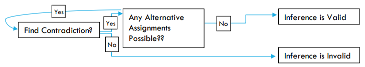
6. If you run into no contradiction, then the inference is invalid because the radioactive row is possible. The process is over.

If you run into a contradiction, then possibly the inference is valid. Complete all lines you’ve started to ensure that there is no possible consistent assignment of truth values. You only need one possible row where there is no contradiction to prove that the inference is invalid; whereas you need to eliminate every possible row that could have true premises and a false conclusion before you can know it’s valid.

Okay, let’s try a more complex one:

Lila: We’re either going home or I’m going home alone unless you both assure me you will drive us home later and will phone the babysitter.

Diego: I can’t assure you that I’ll be sober enough to drive us home later.

Lila: Well, I’m not going home alone and you’re not staying the night here.

Diego: Well, then, I guess either we’re both going home now or we’re getting a motel room.

If we conceive of the whole exchange as one big inference, we can symbolize it the following way:

(H \(\vee\) (I \(\vee\) (A \(\wedge\) P))) / ~A / (~I \(\wedge\) ~S) // (H \(\vee\) M)

Now, we assign truth values to the premises and conclusion so that they’ll be radioactive.

Here, I’ve gone ahead and put them under the main operators:

(H \(\underset{\bf{T}}{\vee}\) (I \(\vee\) (A \(\wedge\) P))) / \(\underset{\bf{T}}{\sim }\)A / (~I \(\underset{\bf{T}}{\wedge}\) ~S) // (H \(\underset{\bf{F}}{\vee}\) M)

Next, I’m going to start looking for some simpler formulas to assign truth values to. I’m eyeing the conclusion and the ~A. The conclusion will only admit of one set of truth values: both H and M must be false for the \(\vee\) to be false. A must be false for ~A to be true.

(H \(\underset{\text{T}}{\vee}\) (I \(\vee\) (A \(\wedge\) P))) / \(\underset{\bf{T}}{\sim }\underset{\text{F}}{A}\) / (~I \(\underset{\text{T}}{\wedge}\) ~S) // (\(\underset{\bf{F}}{H}\underset{\text{F}}{\vee} \underset{\bf{F}}{M}\))

Next, you transfer truth values from the ones you just assigned to all identical letters.

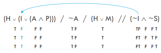
Notice how I’d need the right disjunct (I \(\vee\) (A \(\wedge\) P)) to be true for the first premise to turn out true.

But we already know that A is false from premise 2. So that means the conjunction (A \(\wedge\) P) must be false. Now that we know this, we must conclude that I is true for the first premise to turn out true. So we can conclude that I is true.

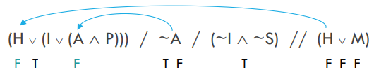
(\(\underset{\text{F}}{H} \underset{\text{T}}{\vee} (\underset{\bf{T}}{I} \vee (\underset{\text{F}}{A} \underset{\bf{F}}{\wedge}\) P))) / \(\underset{\text{T}}{\sim }\underset{\text{F}}{A}\) / (~I \(\underset{\text{T}}{\wedge}\) ~S) // (\(\underset{\text{F}}{H}\underset{\text{F}}{\vee} \underset{\text{F}}{M}\))

Now we transfer the new atomic truth value:

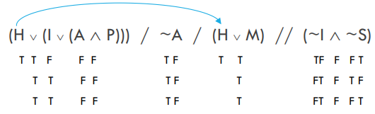
Now let’s try to work out that third premise. First we can process the negation on I:

(\(\underset{\text{F}}{H} \underset{\text{T}}{\vee} (\underset{\text{T}}{I} \vee (\underset{\text{F}}{A} \underset{\text{F}}{\wedge}\) P))) / \(\underset{\text{T}}{\sim }\underset{\text{F}}{A}\) / (\(\underset{\bf{F}}{\sim }\underset{\text{T}}{I} \underset{\text{T}}{\wedge}\) ~S) // (\(\underset{\text{F}}{H}\underset{\text{F}}{\vee} \underset{\text{F}}{M}\))

We’ve already got a contradiction!!! Ouch! ~I would have had to be true for (~I \(\wedge\) ~S) to turn out true. Both conjuncts need to be true. But ~I is false according to our assignment of false to I. Bummer dude!

What now? We’ve reached a contradiction! At this point we ask ourselves: “was there any step I made that I wasn’t forced to make?” In this case, no, we didn’t arbitrarily choose true or false for any letter, so every step we took was forced by logic. That means there aren’t any alternative assignments to consider and therefore the radioactive counterexample is impossible. Our inference is valid.

You could have also assigned values to I and S given the third premise, but I chose to finishing the first premise. Either way would’ve resulted in a contradiction. This is not an example of an alternative assignment. We’ll cover alternative assignments below:

Here's a handy flow chart for you:

Let’s try a quick example with alternative assignments possible:

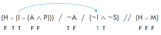
(H \(\underset{\text{T}}{\vee}\) (I \(\vee\) (A \(\wedge\) P))) / \(\underset{\text{T}}{\sim }\)A / (H \(\underset{\text{T}}{\vee}\) M) // (~I \(\underset{\text{F}}{\wedge}\) ~S)

There are many ways for Premise 1 to be true, many ways for Premise 3 to be true, and many ways for the Conclusion to be false (an exception to the generalization I made earlier). So we’re not being forced as much as we were in the previous example. Arguments where the conclusion has more than one way of being false are typically the hardest arguments to do using the reverse truth table method. Hardest, that is, in terms of how much work is involved. Remember that this isn’t difficult in the sense of it being a complicated procedure. It’s not like playing chess. We could program a computer to do this whole method in an afternoon. It does, though, sometimes take a bit of work to work out the answer. Let’s start with what we are forced to do:

(H \(\underset{\text{T}}{\vee}\) (I \(\vee\) (\(\underset{\bf{F}}{A}\) \(\wedge\) P))) / \(\underset{\bf{T}}{\sim }\underset{\text{F}}{A}\) / (H \(\underset{\text{T}}{\vee}\) M) // (~I \(\underset{\text{F}}{\wedge}\) ~S)

A must be false because ~A is true. At this point, we aren’t forced to do anything for Premise 1 since there are still many ways for it to come out true. Nothing has changed for Premise 3 and the Conclusion. At this point we need to split our line into all possible successful assignments. I’m going to start with the conclusion (I chose this more or less arbitrarily). Here’s what I do:

\[\begin{array}{} &(H &\vee (I \vee (&A& \wedge P))) / &\sim &A / (H &\vee M) // (&\sim I& \wedge& \sim S) &&\\ \text{Possibility 1} & \rightarrow &T &F &F &T &F &T &\textbf{T} &F &\textbf{F}&&\\\text{Possibility 2} & \rightarrow &T &F &F &T &F &T &\textbf{F} &F &\textbf{T}&&\\\text{Possibility 3} & \rightarrow &T &F &F &T &F &T &\textbf{F} &F &\textbf{F} && \end{array} \nonumber\]

If you focus on the conclusion, it looks sort of like a truth table now, doesn’t it? Now we complete the process for each possible line:

\[\begin{array}{} (H &\vee (I \vee (&A& \wedge P))) / &\sim &A / (H &\vee M) // (&\sim &I& \wedge& \sim &S) \\& T &F &F &T &F &T &T&\textbf{F} &F &F&\textbf{T}\\ &T &F &F &T &F &T &F&\textbf{T} &F &T&\textbf{F}\\ &T &F &F &T &F &T &F&\textbf{T} &F &F&\textbf{T} \end{array} \nonumber\]

Now I’m transferring truth values:

And then calculate what needs to happen given the changes you’ve made. I’ve changed the first premise, so now I notice that (A \(\wedge\) P) is false and now I is false in my first row, so that means H must be true. In the other rows, nothing has yet forced me to assign anything to H.

\[\begin{array}{} (H &\vee (&I \vee (&A& \wedge P))) / &\sim &A / (H &\vee M) // (&\sim &I& \wedge& \sim &S) \\T& T &F &F &F &T &F &T&T &F &F&F &T\\ &T &T &F &F &T &F &F&F &T &F&T &F\\ &T &T &F &F &T &F &F&F &T &F&F &T \end{array} \nonumber\]

Then transfer that H:

At this point, nothing is forcing my hand. If you look carefully, you’ll see that there is no single letter on any single line that must be a given truth value for the truth values we’ve assigned the complete formulas to obtain. So now what???

If we are free to assign any truth values we want, then we aren’t going to run into any contradictions. It follows that there are no contradictions in these three rows and there is therefore at least one row where there are no contradictions. This inference is invalid.

All we need is one row where there are no contradictions to prove that the inference is invalid.

That’s all! That’s how we do the reverse truth table method. One can imagine how to use this to test even super complex sets of sentences for consistency: just assign “true” to each individual sentence and then look for a contradiction. One line with no contradiction? You’ve got a consistent set of sentences.