2.6: Introduction to Subdivisions in Simple Meters
- Page ID
- 45617
\( \newcommand{\vecs}[1]{\overset { \scriptstyle \rightharpoonup} {\mathbf{#1}} } \)
\( \newcommand{\vecd}[1]{\overset{-\!-\!\rightharpoonup}{\vphantom{a}\smash {#1}}} \)
\( \newcommand{\id}{\mathrm{id}}\) \( \newcommand{\Span}{\mathrm{span}}\)
( \newcommand{\kernel}{\mathrm{null}\,}\) \( \newcommand{\range}{\mathrm{range}\,}\)
\( \newcommand{\RealPart}{\mathrm{Re}}\) \( \newcommand{\ImaginaryPart}{\mathrm{Im}}\)
\( \newcommand{\Argument}{\mathrm{Arg}}\) \( \newcommand{\norm}[1]{\| #1 \|}\)
\( \newcommand{\inner}[2]{\langle #1, #2 \rangle}\)
\( \newcommand{\Span}{\mathrm{span}}\)
\( \newcommand{\id}{\mathrm{id}}\)
\( \newcommand{\Span}{\mathrm{span}}\)
\( \newcommand{\kernel}{\mathrm{null}\,}\)
\( \newcommand{\range}{\mathrm{range}\,}\)
\( \newcommand{\RealPart}{\mathrm{Re}}\)
\( \newcommand{\ImaginaryPart}{\mathrm{Im}}\)
\( \newcommand{\Argument}{\mathrm{Arg}}\)
\( \newcommand{\norm}[1]{\| #1 \|}\)
\( \newcommand{\inner}[2]{\langle #1, #2 \rangle}\)
\( \newcommand{\Span}{\mathrm{span}}\) \( \newcommand{\AA}{\unicode[.8,0]{x212B}}\)
\( \newcommand{\vectorA}[1]{\vec{#1}} % arrow\)
\( \newcommand{\vectorAt}[1]{\vec{\text{#1}}} % arrow\)
\( \newcommand{\vectorB}[1]{\overset { \scriptstyle \rightharpoonup} {\mathbf{#1}} } \)
\( \newcommand{\vectorC}[1]{\textbf{#1}} \)
\( \newcommand{\vectorD}[1]{\overrightarrow{#1}} \)
\( \newcommand{\vectorDt}[1]{\overrightarrow{\text{#1}}} \)
\( \newcommand{\vectE}[1]{\overset{-\!-\!\rightharpoonup}{\vphantom{a}\smash{\mathbf {#1}}}} \)
\( \newcommand{\vecs}[1]{\overset { \scriptstyle \rightharpoonup} {\mathbf{#1}} } \)
\( \newcommand{\vecd}[1]{\overset{-\!-\!\rightharpoonup}{\vphantom{a}\smash {#1}}} \)
\(\newcommand{\avec}{\mathbf a}\) \(\newcommand{\bvec}{\mathbf b}\) \(\newcommand{\cvec}{\mathbf c}\) \(\newcommand{\dvec}{\mathbf d}\) \(\newcommand{\dtil}{\widetilde{\mathbf d}}\) \(\newcommand{\evec}{\mathbf e}\) \(\newcommand{\fvec}{\mathbf f}\) \(\newcommand{\nvec}{\mathbf n}\) \(\newcommand{\pvec}{\mathbf p}\) \(\newcommand{\qvec}{\mathbf q}\) \(\newcommand{\svec}{\mathbf s}\) \(\newcommand{\tvec}{\mathbf t}\) \(\newcommand{\uvec}{\mathbf u}\) \(\newcommand{\vvec}{\mathbf v}\) \(\newcommand{\wvec}{\mathbf w}\) \(\newcommand{\xvec}{\mathbf x}\) \(\newcommand{\yvec}{\mathbf y}\) \(\newcommand{\zvec}{\mathbf z}\) \(\newcommand{\rvec}{\mathbf r}\) \(\newcommand{\mvec}{\mathbf m}\) \(\newcommand{\zerovec}{\mathbf 0}\) \(\newcommand{\onevec}{\mathbf 1}\) \(\newcommand{\real}{\mathbb R}\) \(\newcommand{\twovec}[2]{\left[\begin{array}{r}#1 \\ #2 \end{array}\right]}\) \(\newcommand{\ctwovec}[2]{\left[\begin{array}{c}#1 \\ #2 \end{array}\right]}\) \(\newcommand{\threevec}[3]{\left[\begin{array}{r}#1 \\ #2 \\ #3 \end{array}\right]}\) \(\newcommand{\cthreevec}[3]{\left[\begin{array}{c}#1 \\ #2 \\ #3 \end{array}\right]}\) \(\newcommand{\fourvec}[4]{\left[\begin{array}{r}#1 \\ #2 \\ #3 \\ #4 \end{array}\right]}\) \(\newcommand{\cfourvec}[4]{\left[\begin{array}{c}#1 \\ #2 \\ #3 \\ #4 \end{array}\right]}\) \(\newcommand{\fivevec}[5]{\left[\begin{array}{r}#1 \\ #2 \\ #3 \\ #4 \\ #5 \\ \end{array}\right]}\) \(\newcommand{\cfivevec}[5]{\left[\begin{array}{c}#1 \\ #2 \\ #3 \\ #4 \\ #5 \\ \end{array}\right]}\) \(\newcommand{\mattwo}[4]{\left[\begin{array}{rr}#1 \amp #2 \\ #3 \amp #4 \\ \end{array}\right]}\) \(\newcommand{\laspan}[1]{\text{Span}\{#1\}}\) \(\newcommand{\bcal}{\cal B}\) \(\newcommand{\ccal}{\cal C}\) \(\newcommand{\scal}{\cal S}\) \(\newcommand{\wcal}{\cal W}\) \(\newcommand{\ecal}{\cal E}\) \(\newcommand{\coords}[2]{\left\{#1\right\}_{#2}}\) \(\newcommand{\gray}[1]{\color{gray}{#1}}\) \(\newcommand{\lgray}[1]{\color{lightgray}{#1}}\) \(\newcommand{\rank}{\operatorname{rank}}\) \(\newcommand{\row}{\text{Row}}\) \(\newcommand{\col}{\text{Col}}\) \(\renewcommand{\row}{\text{Row}}\) \(\newcommand{\nul}{\text{Nul}}\) \(\newcommand{\var}{\text{Var}}\) \(\newcommand{\corr}{\text{corr}}\) \(\newcommand{\len}[1]{\left|#1\right|}\) \(\newcommand{\bbar}{\overline{\bvec}}\) \(\newcommand{\bhat}{\widehat{\bvec}}\) \(\newcommand{\bperp}{\bvec^\perp}\) \(\newcommand{\xhat}{\widehat{\xvec}}\) \(\newcommand{\vhat}{\widehat{\vvec}}\) \(\newcommand{\uhat}{\widehat{\uvec}}\) \(\newcommand{\what}{\widehat{\wvec}}\) \(\newcommand{\Sighat}{\widehat{\Sigma}}\) \(\newcommand{\lt}{<}\) \(\newcommand{\gt}{>}\) \(\newcommand{\amp}{&}\) \(\definecolor{fillinmathshade}{gray}{0.9}\)In general, we more accurately gauge shorter periods than longer periods of time. For instance, the difference between the length of whole notes performed at a quarter note = 60 and then at 66 would be difficult to discern. However, we can easily discern the difference between sixteenth notes performed at those speeds, four to a quarter-note beat. Our ability to perceive smaller increments of time can help us with the larger time spans. By accumulating many smaller time spans we can accurate measure or perceive the larger ones.
“Subdivision” or “subdividing” refers to dividing the beat, most often silently, into smaller units. Technically speaking divisions are note values that divide beats (in 4/4 and 6/8 they are eighth notes) and subdivisions are note values that further divide divisions (in 4/4 and 6/8 they are sixteenth notes). Informally, however, most performing musicians use the term subdivision to describe counting note values smaller than the beat. Usually these note values are eighth or sixteenth notes. The ability to subdivide while performing music ensures rhythmic accuracy and is an important skill that all musicians need to develop.
Simple meters (2/4, 3/4, 4/4 etc.) generally feature subdivisions of the beat in four parts. In the figure below please notice that the sixteenth notes form subdivisions of all of the larger value notes:
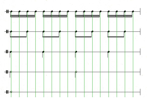
Below is an example with subdivisions: the upper part is aligned with sixteenth note subdivisions in the lower part:
The first step to internalizing the subdivisions is to beat out a steady pattern of sixteenth notes while playing a melody line. For instance, while tapping 16th notes with a hand or foot try singing or saying the upper part with “ta” or “la” for each note. This may take a little bit of practice.
Try tapping out eighth notes while performing these simple patterns:
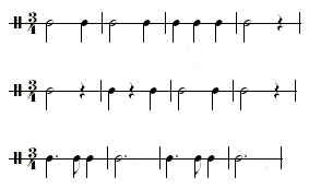
When you are able to perform the rhythms accurately with tapping, try to then perform them accurately by internally “hearing” the taps. When I subdivide I usually do so with internal “tapping” sounds rather than counting “1 ee and ah, 2 ee and ah.” The internal tapping works better with more complex rhythms or faster subdivisions.
When you have mastered the above examples with eighth notes, try subdivisions of sixteenth notes. Here are some further examples to practice with sixteenth note subdivisions:
Choosing Note Values for Subdivisions
Audio engineers speak of “sampling rates,” that is the rate at which sound waves are digitally sampled. The higher the sampling rate, the more accurate is the digital representation of the sound. Similarly in the performance of music, the more subdivisions are made in each beat or each measure, the more exacting the rhythmic performance.
Consider the following figure with notes placed rhythmically placed spatially along the staff line:
If we add eighth note pulses we obtain:
The sixteenth notes at numbers 1 and 2 appear rhythmically accurate; at least they are positioned so that they don’t intersect the eighth note lines. However, if we subdivide the example with sixteenth notes (presented in the green and blue lines) we notice that the rhythmic placement at number 2 is not accurate:
The sixteenth at number 1 coincides with the sixteenth note pulse (blue line) but the sixteenth at number 2 clearly is not centered with the appropriate sixteenth note pulse. The slight rhythmic sloppiness is hardly noticeable with eight note divisions but becomes quite obvious with the sixteenth note subdivisions.
Thus, the smaller and more frequent the rhythmic subdivisions, the more accurately the rhythms can be scrutinized. For this reason, musicians with the highest degree of rhythmic accuracy have the greatest mastery of very rapid subdivisions.
The rule of thumb is to pick the smallest value of subdivision you can internally hear when you perform.