
8.1: What is it?
- Page ID
- 223902

\( \newcommand{\vecs}[1]{\overset { \scriptstyle \rightharpoonup} {\mathbf{#1}} } \)
\( \newcommand{\vecd}[1]{\overset{-\!-\!\rightharpoonup}{\vphantom{a}\smash {#1}}} \)
\( \newcommand{\dsum}{\displaystyle\sum\limits} \)
\( \newcommand{\dint}{\displaystyle\int\limits} \)
\( \newcommand{\dlim}{\displaystyle\lim\limits} \)
\( \newcommand{\id}{\mathrm{id}}\) \( \newcommand{\Span}{\mathrm{span}}\)
( \newcommand{\kernel}{\mathrm{null}\,}\) \( \newcommand{\range}{\mathrm{range}\,}\)
\( \newcommand{\RealPart}{\mathrm{Re}}\) \( \newcommand{\ImaginaryPart}{\mathrm{Im}}\)
\( \newcommand{\Argument}{\mathrm{Arg}}\) \( \newcommand{\norm}[1]{\| #1 \|}\)
\( \newcommand{\inner}[2]{\langle #1, #2 \rangle}\)
\( \newcommand{\Span}{\mathrm{span}}\)
\( \newcommand{\id}{\mathrm{id}}\)
\( \newcommand{\Span}{\mathrm{span}}\)
\( \newcommand{\kernel}{\mathrm{null}\,}\)
\( \newcommand{\range}{\mathrm{range}\,}\)
\( \newcommand{\RealPart}{\mathrm{Re}}\)
\( \newcommand{\ImaginaryPart}{\mathrm{Im}}\)
\( \newcommand{\Argument}{\mathrm{Arg}}\)
\( \newcommand{\norm}[1]{\| #1 \|}\)
\( \newcommand{\inner}[2]{\langle #1, #2 \rangle}\)
\( \newcommand{\Span}{\mathrm{span}}\) \( \newcommand{\AA}{\unicode[.8,0]{x212B}}\)
\( \newcommand{\vectorA}[1]{\vec{#1}} % arrow\)
\( \newcommand{\vectorAt}[1]{\vec{\text{#1}}} % arrow\)
\( \newcommand{\vectorB}[1]{\overset { \scriptstyle \rightharpoonup} {\mathbf{#1}} } \)
\( \newcommand{\vectorC}[1]{\textbf{#1}} \)
\( \newcommand{\vectorD}[1]{\overrightarrow{#1}} \)
\( \newcommand{\vectorDt}[1]{\overrightarrow{\text{#1}}} \)
\( \newcommand{\vectE}[1]{\overset{-\!-\!\rightharpoonup}{\vphantom{a}\smash{\mathbf {#1}}}} \)
\( \newcommand{\vecs}[1]{\overset { \scriptstyle \rightharpoonup} {\mathbf{#1}} } \)
\(\newcommand{\longvect}{\overrightarrow}\)
\( \newcommand{\vecd}[1]{\overset{-\!-\!\rightharpoonup}{\vphantom{a}\smash {#1}}} \)
\(\newcommand{\avec}{\mathbf a}\) \(\newcommand{\bvec}{\mathbf b}\) \(\newcommand{\cvec}{\mathbf c}\) \(\newcommand{\dvec}{\mathbf d}\) \(\newcommand{\dtil}{\widetilde{\mathbf d}}\) \(\newcommand{\evec}{\mathbf e}\) \(\newcommand{\fvec}{\mathbf f}\) \(\newcommand{\nvec}{\mathbf n}\) \(\newcommand{\pvec}{\mathbf p}\) \(\newcommand{\qvec}{\mathbf q}\) \(\newcommand{\svec}{\mathbf s}\) \(\newcommand{\tvec}{\mathbf t}\) \(\newcommand{\uvec}{\mathbf u}\) \(\newcommand{\vvec}{\mathbf v}\) \(\newcommand{\wvec}{\mathbf w}\) \(\newcommand{\xvec}{\mathbf x}\) \(\newcommand{\yvec}{\mathbf y}\) \(\newcommand{\zvec}{\mathbf z}\) \(\newcommand{\rvec}{\mathbf r}\) \(\newcommand{\mvec}{\mathbf m}\) \(\newcommand{\zerovec}{\mathbf 0}\) \(\newcommand{\onevec}{\mathbf 1}\) \(\newcommand{\real}{\mathbb R}\) \(\newcommand{\twovec}[2]{\left[\begin{array}{r}#1 \\ #2 \end{array}\right]}\) \(\newcommand{\ctwovec}[2]{\left[\begin{array}{c}#1 \\ #2 \end{array}\right]}\) \(\newcommand{\threevec}[3]{\left[\begin{array}{r}#1 \\ #2 \\ #3 \end{array}\right]}\) \(\newcommand{\cthreevec}[3]{\left[\begin{array}{c}#1 \\ #2 \\ #3 \end{array}\right]}\) \(\newcommand{\fourvec}[4]{\left[\begin{array}{r}#1 \\ #2 \\ #3 \\ #4 \end{array}\right]}\) \(\newcommand{\cfourvec}[4]{\left[\begin{array}{c}#1 \\ #2 \\ #3 \\ #4 \end{array}\right]}\) \(\newcommand{\fivevec}[5]{\left[\begin{array}{r}#1 \\ #2 \\ #3 \\ #4 \\ #5 \\ \end{array}\right]}\) \(\newcommand{\cfivevec}[5]{\left[\begin{array}{c}#1 \\ #2 \\ #3 \\ #4 \\ #5 \\ \end{array}\right]}\) \(\newcommand{\mattwo}[4]{\left[\begin{array}{rr}#1 \amp #2 \\ #3 \amp #4 \\ \end{array}\right]}\) \(\newcommand{\laspan}[1]{\text{Span}\{#1\}}\) \(\newcommand{\bcal}{\cal B}\) \(\newcommand{\ccal}{\cal C}\) \(\newcommand{\scal}{\cal S}\) \(\newcommand{\wcal}{\cal W}\) \(\newcommand{\ecal}{\cal E}\) \(\newcommand{\coords}[2]{\left\{#1\right\}_{#2}}\) \(\newcommand{\gray}[1]{\color{gray}{#1}}\) \(\newcommand{\lgray}[1]{\color{lightgray}{#1}}\) \(\newcommand{\rank}{\operatorname{rank}}\) \(\newcommand{\row}{\text{Row}}\) \(\newcommand{\col}{\text{Col}}\) \(\renewcommand{\row}{\text{Row}}\) \(\newcommand{\nul}{\text{Nul}}\) \(\newcommand{\var}{\text{Var}}\) \(\newcommand{\corr}{\text{corr}}\) \(\newcommand{\len}[1]{\left|#1\right|}\) \(\newcommand{\bbar}{\overline{\bvec}}\) \(\newcommand{\bhat}{\widehat{\bvec}}\) \(\newcommand{\bperp}{\bvec^\perp}\) \(\newcommand{\xhat}{\widehat{\xvec}}\) \(\newcommand{\vhat}{\widehat{\vvec}}\) \(\newcommand{\uhat}{\widehat{\uvec}}\) \(\newcommand{\what}{\widehat{\wvec}}\) \(\newcommand{\Sighat}{\widehat{\Sigma}}\) \(\newcommand{\lt}{<}\) \(\newcommand{\gt}{>}\) \(\newcommand{\amp}{&}\) \(\definecolor{fillinmathshade}{gray}{0.9}\)Natural deduction is a proof system for propositional logic. In short, it’s a way of proving that really complex argument forms are valid by using really simple argument forms that are easy to understand. In other words, first we learn a series of “rules.” Each rule is an inference that we know is valid. Then we use this method to discover that much more complex arguments are in fact made up of these little arguments we call “rules.” Complex arguments can be proven, in a step-by-step way, to be valid by deriving their conclusions from their premises (by moving step-by-step from just their premises to their conclusions in logically valid steps). If we get from A to B using only valid steps, then the move directly from A to B is itself valid!
Natural deduction is, in practice, a sort of game. We are given some pieces at the beginning (premises), along with rules for how to split apart, combine, and transform those pieces, and we try different strategies until we win the game by making the conclusion. It’s sort of like a puzzle, or a step-by-step strategy game.
Let’s dive right in with an example:
I don’t believe in ghosts, but if I did believe in ghosts, that sound outside would be frightening. Luckily, that sound isn’t frightening to me!
So I guess you really don’t believe in ghosts!
The first step is to symbolize or formalize the argument. This is the process where we take out all of the logically irrelevant content of the argument as it is written here, leaving only the argument structure or form and some symbols which stand in for the content that we took away. This is the first thing we learned in Propositional logic in Chapter 6.
\(\neg\) B \(\wedge\) (B \(\rightarrow\) F)
\(\neg\)F
\(\therefore\) \(\neg\) B
The little “\(\therefore\)” symbol means “therefore” or “what came before is an argument for the following conclusion.”
Now this argument is really clearly valid just by looking at it[1] but it’s helpful to start with a really easy example so that we can build up to the really tricky examples. First, look at the “\(\neg\) B” in the first premise. Notice how it’s identical to the conclusion? Well, anything implies itself deductively. So here’s an argument that is very, very obviously valid:
\(\neg\) B
\(\therefore\) \(\neg\) B
Obviously if “\(\neg\) B” is true, then “\(\neg\) B” must be true. As a matter of absolute necessity. That’s what it means to be valid! Does that make sense?
Now let’s look back at the original argument and try to figure out how it’s valid. This time, I’ll number the premises and put the conclusion off to the side to remind us what we’re looking for. This is exactly the format of a standard natural deduction problem:
1. \(\neg\) B \(\wedge\) (B \(\rightarrow\) F)
2. \(\neg\)F / \(\neg\)B
The numbered propositions 1 and 2 are premises. The “\(\neg\)B” to the right of the slash is the conclusion of the argument. The goal, once we’ve got a problem in front of us, is to move from the premises to the conclusion by means of a set of discrete steps. The moves you can make are determined by which rules you know. We’ll learn some rules soon and that will allow us to make a series of different moves from the premises forward towards the conclusion.
Notice how there are two B’s in premise 1. So, we could take a complex route to proving the conclusion by isolating (getting it by itself) the “(B \(\rightarrow\) F)” and then doing something else to get the B by itself and negating it—adding the “hook” or “\(\neg\)” in front of it. We have B and we want to get to not-B.
Here’s a simpler way, for now:
If I tell you I have an apple and an orange, am I telling you that I have an apple? Yes. Am I telling you that I have an orange? Of course. If, alternatively, I tell you that “if I get into a fender bender on the way to work I’ll be late, but if I don’t, then I’ll have to go to that awful meeting,” am I telling you that “If I get into a fender bender on the way to work then I’ll be late”? Yep! What about “If I don’t get into a fender bender on the way to work, then I’ll have to go to that awful meeting”? Yes again.
So as a general rule, it looks like any time I join two phrases with conjunction, I’m allowed to separate them as well. Every time I tell you something involving ‘but’ or ‘and,’ I’m also telling you that everything on either side of the ‘but’ or ‘and’ is true independently from the rest of the sentence. We’ll talk about this rule more later, but for now we’ll call it simplification, and move on. Let me reiterate, though, that when two things are joined by conjunction, we can just pull them apart in natural deduction and write them all by themselves.
Here’s how we put that rule to use in our example above. I’ll add a new line where I’ve derived a new statement from the existing premises. Our rule “simplification” lets me write something new on its own line. This is how all of the natural deduction rules work: they tell you to find something in the existing propositions and then once you find what you’re looking for, you’re allowed to write something new that the rule tells you to write. What I’m doing here is saying that given those premises (1&2) and all of the simple rules we know, I know it’s logically okay or valid to posit or affirm or state the following (#3) all on its own:
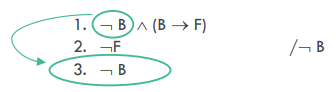
And then I’ll justify that move by appeal to a rule we just learned:
3. \(\neg\) B \(\require{enclose} \enclose{circle}{1, \text{ simplification }}\)
So what I’m communicating here is that I used premise 1 as my “raw material” and applying the rule of simplification to it, which allows me to isolate either the left conjunct (what’s to the left of the wedge or “and” or conjunction symbol) or the right conjunct. I used the rule or operation “simplification” to get “\(\neg\) B” all by itself on a new line. What I’ve said so far is that given premise 1 and the rule “simplification”, we know with deductive certainty that \(\neg\) B is true.
Okay, so that’s one step in. Let’s see how we’re doing:
1. \(\neg\) B \(\wedge\) (B \(\rightarrow\) F)
2. \(\neg\)F / \(\neg\) B
3. \(\neg\) B 1, simplification
Notice at this point that the line we’ve derive—line 3—is exactly identical to the conclusion.
1. \(\neg\) B \(\wedge\) (B \(\rightarrow\) F)
2. \(\neg\)F / \(\enclose{circle}{\neg \text{B }}\)
3. \(\enclose{circle}{\neg \text{B }}\) 1, simplification
This is how we know we’re done with a natural deduction derivation. Why? Well, simply because the whole goal of natural deduction is to derive the conclusion in a set of discrete, understandable steps.
In this case, it turned out to be a very simple derivation because the premises already basically say that B is false, and the conclusion is that B is false. Easy Peasy.
Moving on... We know lots of simple arguments are valid. Maybe we’ve used truth tables or some other simple proof method. Maybe we’ve instead just intuited that a simple argument must be valid like we did above with simplification. Either way, we’ve got a treasure trove of simple argument forms that we can use to prove much more complex argument forms to be valid.
How? Easy! By stringing together a series of simple steps—where each step is deductively valid—that get us from the premises to the conclusion, we will have thereby proven that those premises (or premises of that form) entail or imply with deductive certainty that conclusion (or conclusions of that form). If we can complete a proof like this, then we will have shown that if those premises are true, that conclusion must be true.
[1] That is, if you understand what the symbols means, which you should by now. If you don’t, review the first and second Propositional Logic sections on translation and truth tables. It’s important that you fully understand what each symbol means and can understand their inputs and outputs with ease before moving on to Natural Deduction.