27.3: Picturing Probabilistic and Statistical Structure

We can use simple diagrams to illustrate various probabilistic concepts. Indeed, we can often use them to show why certain probabilistic rules are correct. Some of the diagrams appeared in earlier chapters, but it will be useful to collect them together here and to add a few new tricks.

Probabilities of Disjunctions

We begin with two diagrams we encountered earlier, to remind ourselves how pictures can help us think about probabilities. Recall that a disjunction is an either/or sentence. What is the probability that a disjunction, A or B, has incompatible disjuncts?

Figure \(\PageIndex{1}\): Probabilities of Disjunctions

We can represent the situation with the left subfigure in Figure 27.3.1. To know how much area is covered by either A or by B, we would simply add the two areas together. We represent the fact that the disjuncts are incompatible by a picture in which the two circles representing them do not overlap, so it is easy to see that we didn’t count any portion of the area twice when we added things up.

By contrast, if the disjuncts A and B are compatible, then they can occur together. We represent the fact that they are compatible by a picture in which the two circles representing them do overlap. And this makes it easy to see that if we simply add the area of A to the areas of B, we will count the overlapping (crosshatched) area twice (once when we consider A and a second time when we consider B). The solution is to subtract the probability that A and B both occur so that this area only gets counted once.

We now turn to more difficult problems that are much easier to solve with pictures than with numbers.

Wilbur Fails his Lie Detector Test

The police have word that there is a large conspiracy to sell stolen software. To halt the sales of these stolen goods, they round up a hundred random suspects and give them lie detector tests. Suppose, hypothetically, that the following numbers are correct.

• The machine says a person is lying in 90% of the cases where they really are lying.
• The machine says a person is lying in 20% of the cases where they are not lying.
• 10% of the suspicious characters in town really are guilty. Wilbur failed his test; the machine says he lied. What is the probability that he is guilty?

It is tempting to reason like this: the test is 90% reliable, so there must be about a 90% chance that Wilbur is guilty. The 90% here is the conditional probability of someone’s failing the test if they are guilty.

But this is not what we want to know. We want to know the opposite or inverse of this; we want the probability that someone is guilty, given that they failed. The first figure is Pr(Fails| Guilt), but we want to know the inverse of this, Pr(Guilt |Fails). The two probabilities can be very different; compare: Pr(Male|Pro football player) ≠ Pr(Pro football player |Male)

In the appendix to this chapter we will see how to use our rules to calculate the probability of Wilbur’s guilt. But a simple picture can be used to to solve the problem, and it is much easier to understand.

Figure 27.3.2, which is drawn to scale, represents the relevant information. Remember that there are 100 people in our group.

• 90% of them are not guilty, and they are represented by the wide column on the left of the diagram. Ten percent are guilty, and they are represented by the much thinner column on the right.
• 90% of the guilty people fail the test, and we indicate this with a minus, in 90% of the rows in the thin column.
• 20% of the people who are not guilty fail the test (perhaps they are nervous), and we indicate this with a minus in 20% of the area of the wide, non-guilty column.

Figure \(\PageIndex{2}\): Probability of Guilt Given Test Results

Now we just need to consult the figure and check the percentages. When we do, we find that 9 of the 10 guilty people fail the test, but 18 of the innocent people also fail (18 is 20% of the 90 people who are innocent). So only one person in three who fails the test is guilty. If we have no additional information to go on, the probability that Wilbur is a conspirator is 1/3. It is important that you count, literally, the number of minus signs in the figure to verify this.

Figure \(\PageIndex{3}\): Pie Chart of Lie Detector Test

Similar points apply in many other situations. For example, we may want to know about the probability of having breast cancer, given a small lump and a certain result on a mammogram. Problems like these require us to integrate knowledge about the present case (e.g., what the lie detector says) with prior information about base rates (proportion of guilty people among the suspects). We often focus too much on the present information (Wilbur failed) and ignore information about the base rates of guilty people among the suspects (only 1 in 10).

There are often various ways to display information. We could also depict Wilbur’s plight with a pie chart in which each of our four groups is represented by a slice of the pie (Figure 27.3.3); it is drawn to scale, so that 10% of the pie represents 10% of the group). Such diagrams are often easy to read, but it takes a bit more work to construct them than it does rectangular diagrams.

You should use whatever sorts of pictures you find most helpful, but it is important to construct quick and simple figures; otherwise they will take so much work that (if you are like most of us) you will rarely put in the effort to construct anything at all.

Exercises

1. Draw a picture like that in Figure 27.3.2, and determine the probability of Wilbur’s guilt if all the numbers remain the same, except that the probability of failing the lie detector test if you are not guilty is only 10% (instead of 20%, as above).
2. Draw the picture and determine the probability of Wilbur’s guilt if all the numbers remain the same, except that the base rate of guilty people among the suspicious people is 20% (instead of 10%, as it was above).
3. The staff at the Suicide Prevention Center know that 2% of all people who phone their hot line attempt suicide. A psychologist has devised a quick and simple verbal test to help identify those callers who will attempt suicide. She found that:
   1. 80% of the people who will attempt suicide have a positive score on this test.
   2. But only 5% of those who will not attempt suicide have a positive score on this test.

If you get a positive identification from a caller on this test, what is the probability that they would attempt suicide?

4. Suppose that we have a test for the HIV virus. The probability that a person who really has the virus will test positive is .90, while the probability that a person who does not have it will test positive is .20. Finally, suppose that the probability that a person in the general population has the virus (the base rate of the virus) is .01. Smith’s test came back positive. What is the probability that he really is infected? Construct a diagram to determine the answer (we will work it out by the numbers in the appendix, so you can check your answer against the answer there).

Correlations Revisited

The discussion of correlations in Chapter 15 emphasized pictures, so we will simply recall the basic points here. We saw that the easiest way to understand the basics of correlation is to use a diagram like Figure 27.3.4 on the following page. It depicts four hypothetical relationships between smoking and getting lung cancer. The fact that the percentage line is higher in the smoker’s column than it is in the nonsmoker’s column in the top two diagrams in Figure 27.3.4 indicates that there is positive correlation between being a smoker and having a heart attack. It is the relationship between these two horizontal lines that signifies a positive correlation. And the other diagrams work in the same way. It bears repeating that you do not need to know exact percentages to draw most of these diagrams. You only need to know which column has the higher percentage, i.e., the higher horizontal line.

Figure \(\PageIndex{4}\): Diagrams of Correlations between Smoking and Lung Cancer

Probability Trees

Rectangular diagrams are very clear, but only work well when we are considering two factors, variables, or outcomes. Figure 27.3.5 shows how to represent three variables; here the outcomes of three successive flips of a fair coin, with each flip is a separate variable.

Figure \(\PageIndex{5}\): Tree for Three Variables

In the tree, the numbers along each path represent the probabilities of the outcomes. The probability of a heads on the first flip (represented by the first node of the top path) is 1/2, and the probability of a second heads as we move to the right along that path is also 1/2. There are eight complete paths through the tree, and to assess the probability of any of them (e.g., H1T2H3) we simply multiply the numbers along the path. Since the coin is fair, the probability for each of the eight outcomes represented by the eight full paths is 18.

Trees can also be used when we have fewer than three variables. In Figure 27.3.6, we represent in a tree format the data about Wilbur’s lie detector test that we displayed above in a rectangular diagram. Here we represent the probabilities as labels on the branches.

For example, the branch beginning with Suspects and running to Guilty is labeled 10%, to indicate that 10% of the suspects are guilty. And the bottom branch, from Suspects to Not Guilty, is labeled 90%, to indicate that 90% of the people rounded up are innocent. The additional labels represent the additional probabilities. For example, the top right branch is labeled 10%, to indicate that 10% of the guilty people manage to fool the machine and pass the test.

The arrows point to the number of people who fail the test. There are 9 guilty people who fail plus 18 innocent people who fail, for a total of 27 failed tests. Of these 27 failures 18, or 2/3, are innocent. So, if we have no additional information, our best guess is that the probability that Wilbur is guilty is 1/3.

Figure \(\PageIndex{6}\): Tree Diagram of Wilbur’s Lie Detector Test

Exercises

1. Represent the information about the officials at the Suicide Prevention Center above as a tree and use it to solve the problem.
2. Represent the information about the HIV test above as a tree, and use it to solve the problem.

Brute Enumeration of Percentages

Pictorial Solution to Monty Hall Problem

In the appendix to this chapter we will solve the Monty Hall Problem using probability rules, but most people find a picture of the situation more illuminating. Recall the problem: there are three doors in front of you. There is nothing worth having behind two of them, but there is $1,000,000 behind the third. Pick the right door and the money is yours.

Suppose you choose door 1. But before Monty Hall opens that door, he opens one of the other two doors, picking one he knows has nothing behind it. Suppose he opens door 2. This takes 2 out of the running, so the only question now is about door 1 vs. door 3.

Monty then lets you reconsider your earlier choice: you can either stick with door 1 or switch to door 3. What should you do? More generally, whatever door a person originally picks, should they switch when given the option?

You are better off switching. The basic idea is that when Monte opens one of the two doors you have acquired new information. To represent things pictorially, we begin by figuring out the various things that could occur in this game. You could pick any of the three doors, and the money could be behind any of the three. We represent this situation in Figure 27.3.7 (ignore the thumbs-up signs for now). The first three numbers on the left represent the door you select (either 1, 2, or 3). And for each selection you could make, there are three places where the money could be. So, there are nine possibilities. In the figure, the arrow points to the situation where you selected door 2, but the money was behind door 3.

Figure \(\PageIndex{7}\): Tree of Possible Outcomes in Monty Hall Problem

How to Read the Table

The rows involving switching doors and its outcomes are shaded. Still, Figure 27.3.8 contains a good deal of information so, let’s consider a couple of examples.

• Row one: I picked door 1, and that’s where the money is. Monty can open either door 2 or door 3, since the money isn’t behind either. The only place I can move to is the door he didn’t open. If he opened door 2 I can move to 3; if he opened 3. I can move to 2. In this case, if I switch, I lose.
• Row two: I picked door 2 and the money is behind door 1. The only door Monty can open is door 3. If I stay with door 2 I lose; if I switch to door 1, I win. If I always stick with my original pick, I will win in only 3 of the 9 cases (rows 1, 5, and 9). If I adopt the policy of switching, I will win in 6 of 9 cases (all the other rows). So, I am twice as likely to win the money if I switch. We can present the information more compactly in Figure 27.2.1. Each column indicates what happens in each of the nine situations if I stay or if I switch.

Figure \(\PageIndex{8}\): Using a Picture to Solve the Monte Hall Problem

We can also represent these outcomes with a tree; indeed, the thumbs-up signs in Figure 27.3.9 indicate the cases where you will win if you switch doors. Like our other representations, they show that you double your chances of winning if you switch.

Figure \(\PageIndex{9}\): Simplified Diagram of Monty Hall Problem

As usual, it is helpful to think in terms of proportions or frequencies. Imagine that you play the game many times. What should you expect to happen, on average, every hundred times played? You would win about sixty-six of the hundred games if you switch. You would lose sixty-six if you stick with your original door.

Pictorial Solution to the Two Aces Problem

Remove all the cards except the aces and eights from a deck. This leaves you with an eight-card deck: four aces and four eights. From this deck, deal two cards to a friend. He is honest and will answer exactly one question about his cards. The issue isn’t one about which order in which he got his two cards; indeed, let us suppose he shuffled them before looking at them so that he doesn’t even know which of his cards was dealt first.

1. You ask if his hand contains at least one ace. He answers yes. What is the probability that both of his cards are aces?
2. You ask if his hand contains a red ace. He answers yes. What is the probability that both of his cards are aces?
3. You ask if his hand contains the ace of spades. He answers yes. What is the probability that both of his cards are aces? Using a bit of makeshift but obvious notation, we want to know:

1* Pr(2 aces|at least 1 ace)

2* Pr(2 aces| at least 1 red ace)

3* Pr(2 aces|ace of spades)

All three probabilities are different. We can see the basic point with fewer cards, but the goal here is to examine a problem that needs a little bit bigger diagram than fewer cards would require.

The most difficult part of this problem is figuring out how to represent the various possible hands. We note that there are eight cards one could get on the first draw and seven on the second, so when we take order into account, we have 8 x 7 = 56 hands. Order isn’t relevant here, however, since we aren’t concerned with what card came first, so we can cut 56 in half (counting the outcome of eight of hearts on the first draw and ace of hearts on the second, and the reverse order with the same two cards as the same hand; if you want to consider all 56 cases you can, but it will mean more work).

Indeed, if worst came to worst, you could simply write down all the possible hands in some systematic way, and you would end up with the same 28 hands we’ll begin with here. This takes work in the present case, but with simpler problems it is entirely feasible.

Figure \(\PageIndex{10}\): Diagram for Thinking about Two Aces Problem

There are more efficient ways to solve this problem than by enumerating the hands, but such an enumeration can sometimes give us a better feel for the situation. Such an enumeration is given in Figure 27.3.10, and once we have it, we can determine the answers simply by inspecting the proportions of various sorts of hands (ones with at least one ace, ones with at least one red ace, and so on).

In all three scenarios Wilbur has at least one ace, so only hands with at least one ace are relevant here. A little calculation, or a little trial-and-error doodling, will show that there are 22 hands with at least one ace. Since the ace of spades showed up in the problem, we can begin by enumerating all the two-card hands that contain it. Then we can enumerate those with the ace of hearts, diamonds, and clubs, taking care not to list the same hand twice (if worse comes to worst, you can simply list all the hands and then go through and cross out any duplications).

We are dealing with conditional probabilities, here. Remember how these cut down the set of possibilities (what is sometimes called the sample space). You roll a die and can’t see where it landed. When Wilma verifies it came up an even number, this eliminates all the odd numbers from consideration, and the probability you rolled a two goes up from 1/6 to 1/3. Similarly, when Wilbur tells you he has at least one ace, this eliminates all the hands without any aces, and it also changes various probabilities.

Probability of Two Aces, Given at Least One

First, we’ll see what the probability of Wilbur’s having two aces is, given that he has at least one ace. The 22 hands enumerated in our diagram all contain at least one ace, and 6 of them (those shaded in Figure 27.3.11) have two aces. So, there are 6 ways out of the 22 of having two aces, for a probability of 6/22 (which reduces to 3/11 = .27).

Figure \(\PageIndex{11}\): Two Aces Given at Least One

Probability of Two Aces, Given the Ace of Spades

Now we’ll see what the probability of two aces is, given that one of the cards is the ace of spades. This cuts down the cases we consider—our sample space—to just those hands with the ace of spades. These occupy the first row of our diagram, and there are exactly seven of them. They are enclosed with a dashed line in Figure 27.3.12.

Figure \(\PageIndex{12}\): Two Aces Given the Ace of Spades

Of the seven hands that contain the ace of spades, only three contain two aces (these are enclosed with a solid line and shaded). So, there are 3 two-ace hands out of 7. This yields a probability of 3/7(= 0.43). Hence, the probability of two aces given an ace of spades is substantially higher than the probability of two aces given at least one ace. We leave the last of the three puzzles as an exercise.

Decision Trees

We can often represent situations where we must make a difficult decision with trees. In cases where we have a good estimate of the relevant probabilities and payoffs, we can also represent these on the tree, and use it to help us calculate expected values. Here we will simply note the way in which trees, even in the absence of such information, can help us sort of the relevant alternatives and help us focus those that matter the most.

We will consider a hypothetical example, but situations like this are common; at some point, virtually all of us must make difficult, very possibly life-or-death, decisions about medical treatment, either for our self, or a child or an aging parent. John’s test results are not good. They suggest some possibility of a brain tumor, although the probability is considerably less than 50%. If it is cancer and it’s not surgically removed, John will die in the next year or so. But there is also a genuine risk from the surgery; in a few cases it is fatal, and it leads to lasting damage in other cases. Unless John has the surgery within two months, it will be too late, so the decision needs to be made soon. Of course, John could choose just to not think about it, but this amounts to the decision not to have surgery.

We can represent John’s situation with a tree like that in Figure 27.3.13. This helps us chart the various possibilities. In real life, we rarely can obtain very precise values for probabilities, but in some medical situations a good deal is known about the percentage or proportion of those who have cancer given certain test results or mortality rates in surgeries of a given sort. Where we have these, even if they aren’t completely precise, we can incorporate them into our tree. Such trees can be developed in considerable detail, but we won’t explore them further here.

Figure \(\PageIndex{13}\): Simple Decision Tree

Rectangular Diagrams for Logic and Probability

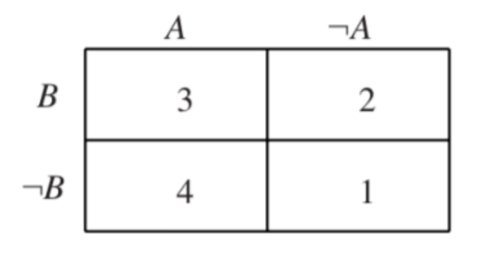
In this section, we develop a simple method for representing important logical and probabilistic relationships with 2 by 2 diagrams. It takes a few minutes practice to become skilled with these diagrams, but it’s a good investment, because it allows us to see many important logical and probabilistic relationships. Where there are only two variables or factors, say A and B, it is often very useful to represent them with a 2 x 2 rectangle like that in Figure 27.3.14.

Columns represent A and its negation ~A.

Rows represent B and its negation ~B.

For easy reference, we can think of these four areas as numbered regions, starting with 1 in the lower right and working our way around (Figure 27.3.14).

Figure \(\PageIndex{14}\): Numbering the Regions

Figure \(\PageIndex{15}\): Areas Corresponding to A and B

In the diagram on the left in Figure 27.3.15, the region with horizontal (leftto-right) hatching (quadrants 3 and 4) represents the area of the rectangle in which A is true. The area with vertical (up-and-down) hatching (quadrants 1 and 2) represents the remaining region where A is false, so the vertical region represents ~A. Similarly, the horizontal region of the diagram on the right in Figure 27.3.15 represents the area where B is true, and the vertical region represents that in which B is false.

Figure \(\PageIndex{16}\): Regions Corresponding to Conjunction and Disjunction

When we are thinking about probability, we interpret the total area of the rectangle as 1. This shows us why the probability of a negation like A will be whatever portion of the unit of probability that isn’t taken by A. A and A must divide the one unit of probability between them, so Pr(~A) = 1-Pr(A).

In the left-hand diagram of Figure 27.3.16 the white, unshaded region (quadrant 3) is where both A and B are true, so it represents the situation where the conjunction, A & B, is true. The remaining, shaded regions (1, 2, and 4) are where this conjunction is false, which is just to say the region where the conjunction’s negation, ~(A & B), is true.

In the right subfigure in Figure 27.3.16, we see that the disjunction, A or B, is true in all the regions except region 1. The white area represents the area where the disjunction is true, so the shaded area represents the area where it is false, i.e., the area (just quadrant 1) where its negation, ~(A or B) is true. But we see that this is also the exact area in which A is false and B is false. After all, A is false in the right-hand column and B is false on the bottom row. And this column and row overlap in the first quadrant. So, this bottom right region is the area where ~A & ~B is true.

Since the regions for ~(A or B) and ~A & ~B coincide (right hand diagram in Figure 27.3.16), they say the same thing. This is a one of two equivalences known as De Morgan’s Laws. In terms of our regions: ~(A or B) = ~A & ~B. The claim that neither A nor B is true is equivalent to the claim that both A and B are false.

There is another, mirror image, version of De Morgan’s laws: ~(A & B) = ~A or ~B. The claim that A and B are not both true is equivalent to the claim that at least one or the other is false.

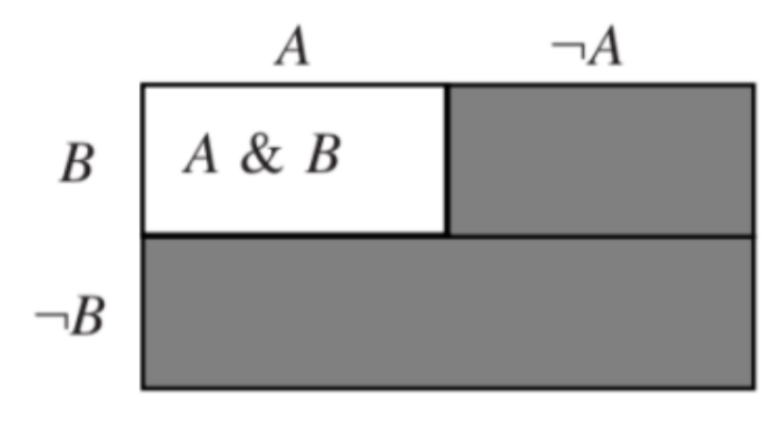
We relabel an earlier diagram as Figure 27.3.17 to illustrate this. Here, the non-shaded region is A & B, so the shaded region is its negation, ~(A & B) (in other words: not both A and B). But with a bit of looking, you can see that this corresponds to the region in which A is false or B is false (or both), i.e., to ~A or ~B

Figure \(\PageIndex{17}\): Shaded: ~( A & B) = ~A or ~B

Equivalence here amounts to two-way validity, so our diagrams show that four separate argument patterns are valid (Figure 27.3.18).

Figure \(\PageIndex{18}\): Four Valid Argument Patterns

We apply all this quite directly to probability by taking the total area of a 2 x 2 rectangle to have the area 1 (representing the total amount of probability). Sentences represented by the same area must have the same probability. Hence, by De Morgan’s Laws, Pr(~(A or B)) = Pr(~A & ~B) and Pr(~(A & B)) = Pr(~A or ~B). We can also use rectangular diagrams to illustrate several of our rules for calculating probabilities. Recall the rule for disjunctions with incompatible disjuncts.

To say that they are incompatible is to say that there is no overlap in their areas of the diagram.

Figure \(\PageIndex{19}\): Rectangular Diagrams for Disjunctions

In the diagram on the left in Figure 27.3.19, A is represented by the horizontal hatching and B by the vertical hatching. Since A and B do not overlap (quadrant 3 is empty), we simply add their probabilities to get the probability for A or B. By contrast, in the diagram on the right in Figure 27.3.19, A and B do overlap, and so when we add their areas, we add A & B (quadrant 3) twice. To make up for this we must subtract it once. Pr(A or B) = Pr(A) + Pr(B) - Pr(A & B).