20.6: Assessing Correlation and Claiming Causation

As we discussed in Chapter 15, it is a common mistake to confuse correlation with causation. In analyzing the data, we get from testing our hypotheses, we are looking to move from mere observation of correlation to understanding causation. How we do that is tricky, though. In this section, we will first look at some complicating factors and outright mistakes people make when looking to claim causation and then we will turn our attention to some methods that work well.

Bad Causal Reasoning

As with other sorts of reasoning, causal reasoning can go awry in many different ways, but there are several patterns of defective causal reasoning that are common enough that we should discuss them here.

Post Hoc, Ergo Propter Hoc

This Latin phrase (usually shortened to ‘post hoc,’ still turns up often enough that it’s worth learning it. It means: after this, therefore because of this. We commit this fallacy when we conclude that A caused B simply because B followed A.

When we put it this way, it is likely to seem like such hopeless reasoning that it isn’t really worth warning about it. Day follows night, but few of us think that day causes night. There are many cases, however, where it really is tempting to reason in this way.

For example, we sometimes take some action, discover the outcome, and conclude that our action led to the outcome. We encountered numerous cases of this sort when we learned about regression to the mean in 16.7.1).

For example, if the institution of a new policy is followed by a decrease in something undesirable or an increase in something desirable, it may be tempting to conclude that the measure caused for the shift. The crime rate went up last year, we added more cops or passed tougher sentencing laws, and this year it came back down to its normal level. In many cases this return to normal might have occurred without the measure, simply as a consequence of regression to the mean. In such cases, we are likely to explain the reduction in crime by the increased number of police or the new laws, but we will be wrong, and the new measure will be given credit it doesn’t deserve.

As a final example, when some people recover from a given illness after taking a certain drug, it is tempting to conclude that the drug caused their recovery. But might they have recovered anyway, without the drug? In many cases, people do. Here we need to compare the rate of recovery among those who take the drug with the rate among those who do not. In many cases, the best way to do this is with a controlled experiment. The connection here may just be an illusory correlation (Chapter 15), and if it is, there is no interesting causal connection here at all.

Figure \(\PageIndex{1}\): Common Causes

Common Causes

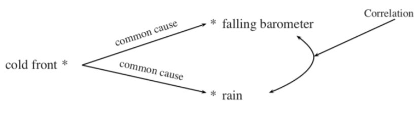
When two sorts of things are positively correlated, it is sometimes the case that one causes the other. But we reason badly when we take a correlation between two things to show that one causes the other. When we studied samples and correlations (Chapter 15) we noted that correlations between two things are often based on some third, common cause. For example, there is a positive correlation between a falling barometer and a rainstorm, but neither causes the other. They are the joint effects of a common cause: an approaching cold front.

Separating Cause from Effect

Sometimes the problem here is described as confusing cause and effect. How could anyone have a problem with this? Isn’t it usually obvious? Yes, very often it is. But in complex systems it is often difficult to determine what causes what.

Families with a member who is schizophrenic tend to be dysfunctional in various ways. But does the schizophrenia lead to familial problems or do the problems lead to the schizophrenia? The answer needn’t be simple. In addition to these two possibilities, it may be that there is some third, common, cause. Or it may be that each thing makes the other worse. There may be a sort of vicious circle with a feedback loop.

Feedback Loops

Feedback loops occur when the output of a system is then used as input for the same system. These loops make it tricky to engage in causal reasoning because they entangle cause and effect. Take for example temperature change and melting snow and ice. As temperatures increase snow and ice melt, which reveals more earth. The exposed ground is less reflective and absorbs more heat, causing temperatures to rise, which itself causes more snow to melt. We end up with a system where rising temperatures melts snow and ice, but melting snow and ice cause temperatures to rise. So, which is the cause, and which is the effect? That way of thinking is wrongheaded because of the feedback loop. The only correct way to understand causation in this case is by looking at the system as a whole and seeing them as entangled.

Confounding Variables

In other cases, a number of things go together in ways that may make it difficult to determine exactly what causes what. For example, people of color receive worse health care, as a group, than white people. But it is sometimes argued that this isn’t a direct result of racial discrimination but of economic differences (which often are a result of discrimination), lack of good health insurance, or yet other factors. The more involved a system is, the more complicated things are, and the less likely it is that any single cause can be identified (although in the above example, it is going to be the case that addressing discrimination and systemic injustice would address much of the problem).

Causal Schemas

One final aspect of bad causal reasoning to keep in mind is the existence of causal schemas. A Causal schema is a cognitive short cut that we have developed to help us explain commonplace cause and effect. If your mom always cooks you breakfast in the morning, and you wake up and see breakfast on the table, you will immediately conclude that your mother was the cause of breakfast. We rely on causal schemas all the time. If we didn’t, we would constantly be starting from scratch trying to figure out how we find ourselves in the situations we are in. Taking into account the information cost of reinvestigating everything all of the time causal schemas are necessary in everyday life.

When we really need to understand cause and effect, though, casual schemas can get in the way of the truth. This is because the whole purpose of causal schemas is to allow us to skip investigation, but the only way we can know is if we investigate. Consider the breakfast example above. While your mother is the person who has always prepared breakfast in the past, it is possible that your father, sibling, or a bizarre home invader made the meal. It is also important to keep in mind that our causal schemas are only as good as the investigation that went into forming them in the first place. Inaccurate beliefs lead to inaccurate schemas.

Mill’s Methods

Mill’s methods are techniques designed to help us isolate the genuine causes from a list of potential causes. They are often called eliminative because they pinpoint the true cause (when they do) by eliminating potential causes that aren’t genuine. These techniques get their name from John Stuart Mill (1806–1874), the British philosopher who systematized them. They weren’t invented by Mill, though, since people who engaged in careful causal reasoning always employed similar strategies.

Mill’s methods are not magical. They cannot pinpoint causes in a vacuum. They require us to make substantive assumptions about the sorts of things that might have caused a given event or type of event. In many situations we can do this with a reasonable degree of confidence, so the methods are often useful. But they are not foolproof; causal reasoning is inductive reasoning, and so it is subject to standard inductive uncertainty. To that end we need to remember, as always, to remain fallible about the conclusions that we draw using these methods.

Method of Agreement

Basic Idea: We need to focus on things that are the same, that agree between cases. If a potential cause A is present when an effect E is absent, then A isn’t the cause of E. If we can eliminate all but one of the potential causes in cases where E occurs, then the remaining potential cause is the actual or genuine cause.

Examples

Bad Oysters: You and several friends get sick after going out to eat together. You each had different entrées and cocktails, but you shared the raw oyster appetizer. You can eliminate all food and drinks you didn’t all have as causes for the food poisoning.

Toxic Relationships: Every relationship Steve has been in is unhealthy. Steve and his various partners fight until eventually they break up. The thing common in all of the toxic relationships is Steve. We are left to conclude Steve is the cause of the relationship problems.

Method of Difference

Basic Idea: We need to focus on what is different between cases. If an effect of interest occurs in one case but not in a second, look for a potential cause that is present in the first case but not in the second. If you find one, it is likely to be the cause (or at least part of the cause).

Examples

Getting your car to start: If your car started yesterday but won’t start today, we need to think about what might have changed. If it was 50 degrees yesterday and today it is 20 degrees, it might be that the colder temperature is preventing your car from starting.

Allergic reaction: You go into your backyard to enjoy the beautiful flowers that your partner has planted. Before long, your eyes begin to water, and your nose starts to run. You go back inside. Soon, the symptoms subside. It is likely that the difference in your environment – flowers versus no flowers – were causing your symptoms.

Baking a Cake: If the first time you made a cake it was pretty good, and the second time not so much, you should think about what you did different. If you decided to substitute salt for sugar the second time, that difference is likely to be the cause of it tasting less good.

Joint Method of Agreement and Difference

Basic Idea: We are combining the previous two methods. So, we are looking to see what is different between cases with different outcomes and what is the same about the ones that have the same outcome. If A is always present when, but only when, E is present, then A caused E. When agreement and difference were considered apart, we could conclude likelihood of causation in each case. Now that we have combined them, it seems even more likely we can conclude causation because A looks to be necessary and sufficient for E.

Examples

Test Prep: All the people who took the Wilburton Prep course for the LSAT (a test used in making decisions about admissions to law schools) were accepted by the law school they wanted to attend. But none of the people who applied to the same law school but didn’t take the course were accepted.

Bad Oysters Part II: This time everyone decides to order the same entrées and cocktails, but after the bad experience last time only half of you ate the raw oyster appetizer. Again, some of you get sick. It turns out only the people who ate the appetizer got sick. Now you can see that everyone who ate the raw oysters got sick and nobody who didn’t got sick.

Toxic Relationships Part II: Every relationship Steve has been in is unhealthy. Steve and his various partners fight until eventually they break up. After moving on from Steve, all his partners find themselves in loving healthy relationships. The thing common in all the toxic relationships is Steve, and once Steve is absent the toxicity does not manifest. We now have more evidence that Steve is the cause of the relationship problems.

Method of Residues

Basic Idea: Sometimes we have a complicated situation with several causes and outcomes. If a number of factors are thought to cause a number of outcomes and all of the factors have been matched to outcomes except one, then the remaining factor can be understood as the cause of the last outcome. Basically, we can disentangle things by narrowing our focus to the things left in the group that have not been matched.

Example

Sick at the Fair: You notice that every year after attending the State Fair you have a stomachache, you’re woozy and light-headed, and your skin feels very hot. You think about what a day at the Fair is normally like for you. It seems that your day at the fair invariably falls on a hot, sunny day which is too bad, since there’s very little shade and you never remember to wear sunscreen. The bathroom situation is always disgusting, so you avoid drinking as much as possible, to avoid having to use it, but you do spend the day stuffing yourself with deep-fried everything.

So, you have three symptoms, a stomachache, light-headedness and a sunburn and three causes, long hours in the sun, gorging on greasy food and not drinking water. You quickly piece together that the greasy food caused the stomachache and the hot sun lead to the sunburn. As they are the only things left, the failure to drink water must have caused the light-headedness (although you might notice that there is also a feedback loop at play, here, as the hot sun that lead to the sunburn also accelerated the dehydration when you didn’t drink).

Method of Concomitant Variation

Basic Idea: This method is related to our earlier discussion of correlation (Chapter 15). It is relevant when different amounts or rates of something are involved. The word ‘concomitant’ is not as common as it was in Mill’s day, but it simply means accompanying. This method applies when an increase in one variable is accompanied by an increase in the other. If the amount of outcome E increases as the amount of event A increases, then A likely causes E.

Examples

Cigarettes: Aiko has recently started smoking. She has found that the more cigarettes she smokes, the more headaches she has. The method of concomitant variation tells us the cigarettes are the likely cause of the headaches.

Podcast: A few months ago, Aadesh found a new podcast he likes. He has gone from listening occasionally to consuming the hundreds of past episodes and new ones as soon as they come out. Over this same time, people close to Aadesh observe that he has begun to make misogynistic comments with increasing frequency, proportional to the amount of time he spends listening to the podcast. The method of concomitant variation tells us that the podcast is amping up Aadesh’s misogynistic rhetoric.