15.3: Correlation

Some variables tend to be related. Taller people tend to weigh more than shorter people. People with more education tend to earn more than people with less. Smokers tend to have more heart attacks than non-smokers. There are exceptions, but “on average” these claims are true.

There are many cases where we want to know the extent to which two variables are related. What is the relationship between the number of cigarettes someone smokes and their chances of getting lung cancer? Is there some relationship between years of schooling and average adult income? What is the connection between class attendance and grades in this course? Learning the answers to such questions is important for discovering how to achieve our goals (“Since the chances of getting cancer go up a lot, I’ll try to quit smoking even though I really enjoy it.”).

Correlation is a measure of the degree to which two variables are related— the degree to which they vary together (“covary”). If two things tend to go together, then there is a positive correlation between them. For example, the height and weight of people are positively correlated; in general, greater height means greater weight. On the other hand, if two things tend to vary inversely there is a negative correlation between them. For example, years of schooling and days spent in prison are negatively correlated; in general, more years of schooling means less time in jail. And if two things are completely unrelated, they are not correlated at all.

Correlations between variables are extremely important in prediction. If you knew the heights of all the students in your critical reasoning class, you would be able to make more accurate predictions about each student’s weight than if you didn’t know their heights. You would still make some mistakes, but on average your predictions would be more accurate.

There is a formula for calculating correlations, and the resulting values are numbers between +1.0 (for complete positive correlation) and 10 (for a complete negative correlation); a correlation of 0 means that there is no pattern of relationship between the two variables. This allows for very precise talk about correlations. We won’t worry about such precision here, however, but will simply focus on the basic ideas.

Correlation and Probability

We could apply the things we learned about probability to cover all cases of correlation, but here we will just get the general idea by considering the case of two dichotomous variables (variables that only have two values).

Consider the smoking variable and its two values, smoker and non-smoker, and the heart-attack variable and it’s two values, having a heart attack and not having a heart attack. The two variables are not independent. Smokers are more likely than non-smokers to have heart attacks, so there is a positive correlation between smoking and heart attacks. This means that Pr(H|S) > Pr(H) > Pr(H |~S). Or in words, the property of having a heart occurs at a higher rate in one group (smokers) than in another group (people in general, as well as the group of people who don’t smoke). So, correlation compares the rate at which a property (like having a heart attack) occurs in two different groups.

If the correlation were negative, we would instead have Pr(H|S) < Pr(H). And if there were no correlation at all, the two variables would be independent of each other, i.e., Pr(H|S) = Pr(H). Correlation is symmetrical. That means that it is a two-way street. If S is positively correlated with H, then H is positively correlated with S, and similarly for negative correlations and for non-correlations. In terms of probabilities this means that if Pr(A|B) > Pr(A), then Pr(B|A) > Pr(B) (exercise for experts: prove this).

Correlation is Comparative

The claim that there is a positive correlation between smoking and having a heart attack does not mean that a smoker is highly likely to have a heart attack. It does not even mean that a smoker is more likely than not to have a heart attack. Most people won’t have heart attacks even if they do smoke.

The claim that there is a positive correlation between smoking and having a heart attack simply means that there are more heart attack victims among smokers than among non-smokers.

Figure \(\PageIndex{1}\): Thinking about Correlations

A good way to get a rough idea about the correlation between two variables is to fill in some numbers in the table in Figure 15.3.1. It has four cells. The + means the presence of a feature (smoking, having a heart attack) and the - means not having that feature (being a non-smoker, not having a heart attack). So, the cell at the upper left represents people who are both smokers and suffer heart attacks, the cell at the lower left represents people who are non-smokers but get heart attacks anyway, and so on. We could then do a survey and fill in numbers in each of the four cells.

The key point to remember is that smoking and heart attacks are correlated just in case Pr(S|H) > Pr(S|~H). So, you cannot determine whether they are correlated merely by looking at Pr(S|H). This number might be high simply because the probability of suffering a heart attack is high for everyone, smokers and nonsmokers alike. Correlation is comparative: you must compare Pr(S|H) to Pr(S|~H) to determine whether smoking and heart attacks are correlated or not.

Figure \(\PageIndex{2}\): Correlation between Smoking and Heart Attacks

Comparative Diagrams to Illustrate Correlation

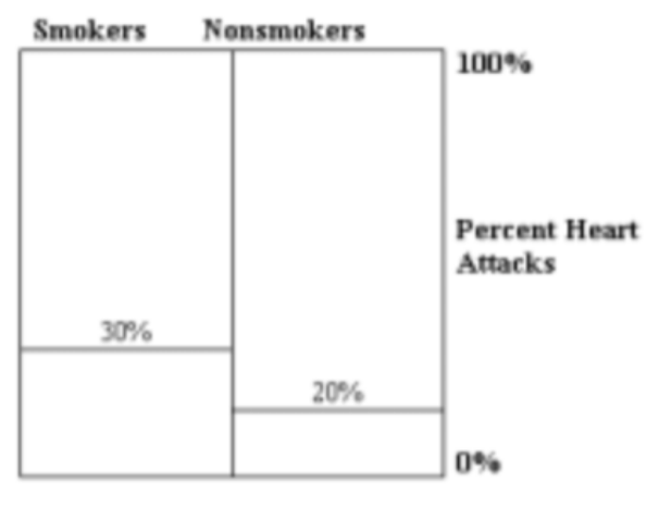
One of the easiest ways to understand the basics of correlation is to use a diagram like that in Figure 15.3.2. Diagrams like this are more rough and ready than the diagram above, but they are easier to draw. The percentages are hypothetical and are simply used for purposes of illustration. Here we suppose that the percentage of smokers who suffer heart attacks is 30%, and that the percentage of nonsmokers who suffer heart attacks is 20% (these round numbers are chosen to make the example easier; they are not the actual percentages).

In this comparative diagram, the horizontal line in the smokers column indicates that 30% of all smokers suffer heart attacks, and the lower horizontal line in the nonsmokers column indicates that 20% of nonsmokers suffer heart attacks.

Figure \(\PageIndex{3}\): A Stronger Positive Correlation

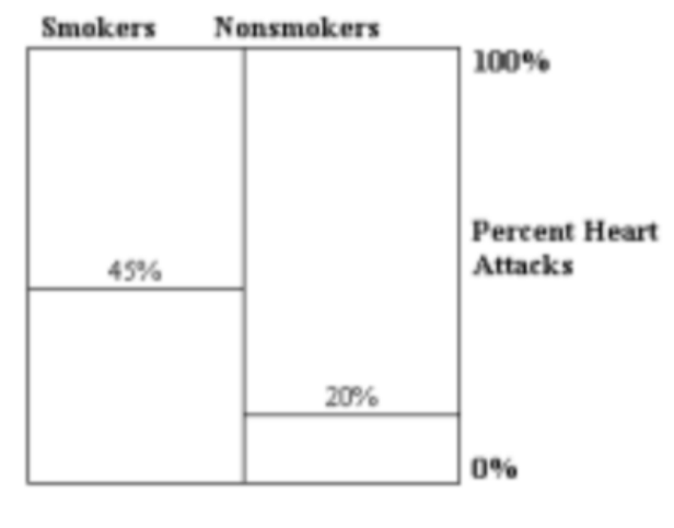
The fact that the percentage line is higher in the smokers column than it is in the nonsmokers column indicates a positive correlation between being a smoker and having a heart attack. It is the relationship between these two horizontal lines that signifies a positive correlation. Similarly, the fact that the percentage line is lower in the nonsmokers column indicates that there is a negative correlation between being a nonsmoker and having a heart attack. The further apart the lines are in a diagram like this, the stronger the correlation. So, Figure 15.3.3 illustrates an even stronger positive correlation between smoking and heart attacks.

Figure \(\PageIndex{4}\): Independence between Smoking and Heart Attacks

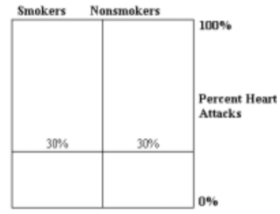
Finally, if the lines were instead the same height, say at 30% (as in Figure 15.3.4), smoking and having a heart attack would be independent of one another: they would not be correlated, either positively or negatively.

Notice that to draw such diagrams you do not need to know exact percentages. You only need to know which column should have the higher percentage, i.e., the higher horizontal line.

Correlation and Causation

Correlations often point to causes; they are evidence for claims about what causes what. When two variables, like smoking and having a heart attack, covary we suspect that there must be some reason for their correlation— surely something must cause them to go together. But correlation is not the same thing as causation. For one thing, correlation is symmetrical (smoking and heart attacks are correlated with each other), but causation is a one-way street (smoking causes heart attacks, but heart attacks rarely cause people to smoke). So, just finding a positive correlation doesn’t tell us what causes what.

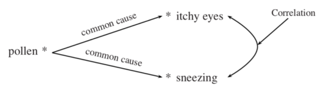
When your child’s pediatrician says, “Spots like this usually mean measles,” they are relying on a positive correlation between the presence of spots and having measles. We know the spots don’t cause the measles, and commonsense suggests that measles causes the spots. But sometimes variables are correlated with each other even when neither has any causal influence on the other. For example, every spring my eyes start to itch and a day or two later I have bouts of sneezing. But the itchy eyes don’t cause the sneezing; these two symptoms are joint effect of a third factor, allergies to pollen, that causes them both (Figure 15.3.5).

Similarly, there is a positive correlation between a falling barometer and a rainstorm, but neither causes the other. They are both caused by an approaching cold front. So, sometimes variables are correlated because they have a common cause, rather than because either causes the other. There are many examples of correlations between things that are effects of some third, common cause. The scores of identical twins reared in very different environments are correlated on multiple behavioral variables like introversion– extroversion. If the twins were separated at birth and reared apart, one twin’s high degree of extroversion cannot be the cause of the other’s extroversion. In this case, their high degrees of extroversion are joint effects of a third thing—a common cause—namely having the same genotype (genetic makeup).

Figure \(\PageIndex{5}\): Common Causes

Some early spokesmen (they were all men in those days) for the tobacco companies tried to convince the public that something similar was true in the case of smoking. They urged that smoking and heart attacks are correlated because they are common effects of some third factor. Some peoples’ genetic makeup, the spokesmen suggested, both led them to smoke and made them more susceptible to heart disease. Despite much research, a common genetic cause for smoking and cancer was never found, but the research was necessary to exclude this possibility. We can never rule out the possibility of common causes without empirical observations.

In many cases, it is difficult to determine what causes what, even when we know a lot about correlations. For example, in the late 1990s, the rate of violent crime in many U. S. cities dropped. The drop was accompanied by several factors, e.g., more police on the beat, tougher sentencing laws, various educational programs. Thus, there is a (negative) correlation between number of police and number of crimes, between tougher sentences and number of crimes (more police, less crime), and so on. But there is a great deal of debate about just what caused the crime drop (naturally, everyone involved wants to take credit for it). Of course, it may be that each of these factors, e.g., more police, increased education, played some causal role. It is very difficult to determine just how much difference each of the factors makes, but we need to do so, if we are going to implement effective measures to reduce crime.

It is also known that self-esteem and depression are negatively correlated. Lower self-esteem tends to go with depression. But what causes what? Lower self-esteem might well lead to depression, but depression might also lower self-esteem. Of course, there could be a vicious circle here, where each condition worsens the other. But it is also possible that there is some third cause, e.g., a low level of neurotransmitters in the brain, or negative events in one’s life.

As these examples show, finding causes is often important for addressing serious problems like crime and depression. But while correlations can frequently be detected by careful observation, tracking down causes is often much more difficult. It is best done in an experimental setting, where we can control for the influence of the relevant variables.

Correlation and Inferential Statistics

Once we determine whether two variables are correlated in a sample, we may want to draw inferences about whether they are correlated in the population. Here, the material earlier in this chapter on inferential statistics is relevant.

Exercises

1. Identify whether the correlation between the following pairs of variables is strong, moderate, or weak, and in those cases that do not involve dichotomous variables, identify whether the correlation is positive or negative. Defend your answer (if you aren’t sure about the answer, explain what additional information you would need to discover it); in each case, think of the numbers as measuring features of adults in the United States:
   1. height and weight
   2. weight and height
   3. weight and caloric intake
   4. weight and income
   5. weight and score on the ACT
   6. weight and amount of exercise
   7. weight and gender
   8. years of schooling and income
2. Having schizophrenia and being from a dysfunctional family are positively correlated. List several possible causes for this correlation. What tests might determine which possible causes are really at play?
3. How might you determine whether watching television shows depicting violence and committing violent acts are correlated in children under ten? Suppose that they were: what possible causes might explain this correlation?
4. Many criminals come from single parent homes. Explain in detail what you would need to know to determine whether there really is a correlation between being a criminal and coming from a single parent home. Then explain what more you would need to know to have any sound opinion on whether coming from a single parent home causes people to become criminals.
5. How would you go about assessing the claim that there is a strong positive correlation between smoking marijuana and getting in trouble with the law?
6. We often hear about the power of positive thinking, and how people who have a good, positive attitude have a better chance of recovering from many serious illnesses. What claim does this make about correlations? How would you go about assessing this claim?
7. Suppose that 30% of those who smoke marijuana get in trouble with the law, and 70% do not. Suppose further that 27% of those who don’t smoke marijuana get in trouble with the law and 73% do not. What are the values of Pr(T|M) and Pr(T|~M). Are smoking marijuana and getting in trouble with the law correlated? If so, is the correlation positive or negative? Does it seem to be large or small?
8. Suppose we obtain the following statistics for Wilbur’s high school graduation class: 46 of the students (this is the actual number of students, not a percentage) who smoked marijuana got in trouble with the law, and 98 did not. And 112 of those who didn’t smoke marijuana got in trouble with the law and 199 did not. What are the values of Pr(T|M) and Pr(T|~M)? Are smoking marijuana and getting in trouble with the law correlated? If so, is the correlation positive or negative? Does it seem to be large or small?
9. Suppose that last year the highway patrol in a nearby state reported the following: 10 people who died in automobile accidents were wearing seatbelts and 37 were not wearing seatbelts. Furthermore, 209 people who did not die (but were involved) in accidents were wearing their seatbelts, while 143 were not wearing them. Does this give some evidence that seatbelts prevent death in the case of an accident? Is there a non-zero correlation between wearing seat belts and being killed in an accident? If so, is it positive or negative, and what is the relative size (large, moderate, small)? Be sure to justify your answers.

Extras for Experts. Prove that positive correlation is symmetrical. That is, prove that Pr(A|B) > Pr(A) just in case Pr(B|A) > Pr(B)