5.5: Statistical Reasoning- Bayes’ Theorem

Frequency diagrams: A first look at Bayes

Bayesian reasoning is about how to revise our beliefs in the light of evidence. We'll start by considering one scenario in which the strength of the evidence has clear numbers attached. (Don't worry if you don't know how to solve the following problem. We'll see shortly how to solve it.)

Suppose you are a nurse screening a set of students for a sickness called Diseasitis.1

• You know, from past population studies, that around 20% of the students will have Diseasitis at this time of year.

You are testing for Diseasitis using a color-changing tongue depressor, which usually turns black if the student has Diseasitis.

• Among patients with Diseasitis, 90% turn the tongue depressor black.
• However, the tongue depressor is not perfect, and also turns black 30% of the time for healthy students.

One of your students comes into the office, takes the test, and turns the tongue depressor black. What is the probability that they have Diseasitis?

(If you think you see how to do it, you can try to solve this problem before continuing. To quickly see if you got your answer right, you can expand the "Answer" button below; the derivation will be given shortly.)

The probability a student with a blackened tongue depressor has Diseasitis is 3/7, roughly 43%. This problem can be solved a hard way or a clever easy way. We'll walk through the hard way first.

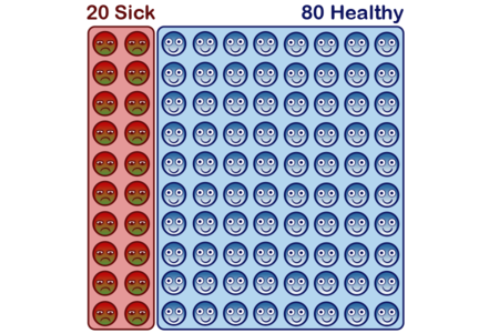
First, we imagine a population of 100 students, of whom 20 have Diseasitis and 80 do not.2

90% of sick students turn their tongue depressor black, and 30% of healthy students turn the tongue depressor black. So we see black tongue depressors on 90% * 20 = 18 sick students, and 30% * 80 = 24 healthy students.

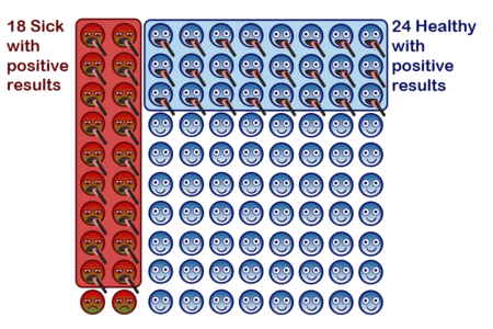
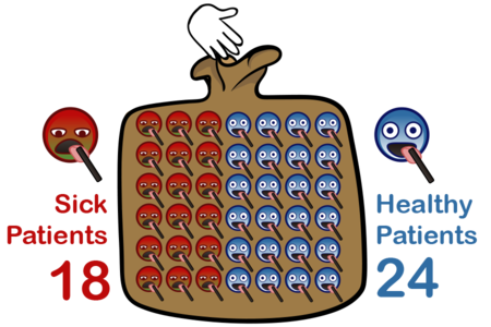
What's the probability that a student with a black tongue depressor has Diseasitis? From the diagram, there are 18 sick students with black tongue depressors. 18 + 24 = 42 students in total turned their tongue depressors black. Imagine reaching into a bag of all the students with black tongue depressors, and pulling out one of those students at random; what's the chance a student like that is sick?

The final answer is that a patient with a black tongue depressor has an 18/42 = 3/7 = 43% probability of being sick.

Many medical students have at first found this answer counter-intuitive: The test correctly detects Diseasitis 90% of the time! If the test comes back positive, why is it still less than 50% likely that the patient has Diseasitis? Well, the test also incorrectly "detects" Diseasitis 30% of the time in a healthy patient, and we start out with lots more healthy patients than sick patients.

The test does provide some evidence in favor of of the patient being sick. The probability of a patient being sick goes from 20% before the test, to 43% after we see the tongue depressor turn black. But this isn't conclusive, and we need to perform further tests, maybe more expensive ones.

If you feel like you understand this problem setup, consider trying to answer the following question before proceeding: What's the probability that a student who does not turn the tongue depressor black - a student with a negative test result - has Diseasitis? Again, we start out with 20% sick and 80% healthy students, 70% of healthy students will get a negative test result, and only 10% of sick students will get a negative test result.

Imagine 20 sick students and 80 healthy students. 10% * 20 = 2 sick students have negative test results. 70% * 80 = 56 healthy students have negative test results. Among the 2+56=58 total students with negative test results, 2 students are sick students with negative test results. So 2/58 = 1/29 = 3.4% of students with negative test results have Diseasitis.

Now let's turn to a faster, easier way to solve the same problem.

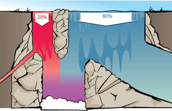
Imagine a waterfall with two streams of water at the top, a red stream and a blue stream. These streams separately approach the top of the waterfall, with some of the water from both streams being diverted along the way, and the remaining water falling into a shared pool below.

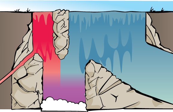
Suppose that:

• At the top of the waterfall, 20 gallons/second of red water are flowing down, and 80 gallons/second of blue water are coming down.
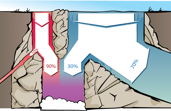
• 90% of the red water makes it to the bottom.
• 30% of the blue water makes it to the bottom.

Of the purplish water that makes it to the bottom of the pool, how much was originally from the red stream and how much was originally from the blue stream?

This is structurally identical to the Diseasitis problem from before:

• 20% of the patients in the screening population start out with Diseasitis.
• Among patients with Diseasitis, 90% turn the tongue depressor black.
• 30% of the patients without Diseasitis will also turn the tongue depressor black.

The 20% of sick patients are analogous to the 20 gallons/second of red water; the 80% of healthy patients are analogous to the 80 gallons/second of blue water:

The 90% of the sick patients turning the tongue depressor black is analogous to 90% of the red water making it to the bottom of the waterfall. 30% of the healthy patients turning the tongue depressor black is analogous to 30% of the blue water making it to the bottom pool.

Therefore, the question "what portion of water in the final pool came from the red stream?" has the same answer as the question "what portion of patients that turn the tongue depressor black are sick with Diseasitis?"

Now for the faster way of answering that question.

We start with 4 times as much blue water as red water at the top of the waterfall.

Then each molecule of red water is 90% likely to make it to the shared pool, and each molecule of blue water is 30% likely to make it to the pool. (90% of red water and 30% of blue water make it to the bottom.) So each molecule of red water is 3 times as likely (0.90 / 0.30 = 3) as a molecule of blue water to make it to the bottom.

So we multiply prior proportions for red vs. blue by relative likelihoods of and end up with final proportions that mean that the bottom pool has 3 parts of red water to 4 parts of blue water.

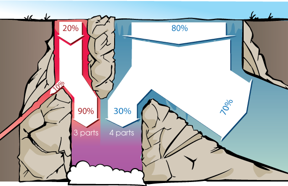
To convert these relative proportions into an absolute probability that a random water molecule at the bottom is red, we calculate 3 / (3 + 4) to see that 3/7ths (roughly 43%) of the water in the shared pool came from the red stream.

This proportion is the same as the 18 : 24 sick patients with positive results, versus healthy patients with positive test results, that we would get by thinking about 100 patients.

That is, to solve the Diseasitis problem in your head, you could convert this word problem:

20% of the patients in a screening population have Diseasitis. 90% of the patients with Diseasitis turn the tongue depressor black, and 30% of the patients without Diseasitis turn the tongue depressor black. Given that a patient turned their tongue depressor black, what is the probability that they have Diseasitis?

Okay, so the initial odds are (20% : 80%) = (1 : 4), and the likelihoods are (90% : 30%) = (3 : 1). Multiplying those ratios gives final odds of (3 : 4), which converts to a probability of 3/7ths.

(You might not be able to convert 3/7 to 43% in your head, but you might be able to eyeball that it was a chunk less than 50%.)

You can try doing a similar calculation for this problem:

• 90% of widgets are good and 10% are bad.
• 12% of bad widgets emit sparks.
• Only 4% of good widgets emit sparks.

What percentage of sparking widgets are bad? If you are sufficiently comfortable with the setup, try doing this problem entirely in your head.

(You might try visualizing a waterfall with good and bad widgets at the top, and only sparking widgets making it to the bottom pool.)

• There's (1 : 9) bad vs. good widgets.
• Bad vs. good widgets have a (12 : 4) relative likelihood to spark.
• This simplifies to (1 : 9) x (3 : 1) = (3 : 9) = (1 : 3), 1 bad sparking widget for every 3 good sparking widgets.
• Which converts to a probability of 1/(1+3) = 1/4 = 25%; that is, 25% of sparking widgets are bad.

Seeing sparks didn't make us "believe the widget is bad"; the probability only went to 25%, which is less than 50/50. But this doesn't mean we say, "I still believe this widget is good!" and toss out the evidence and ignore it. A bad widget is relatively more likely to emit sparks, and therefore seeing this evidence should cause us to think it relatively more likely that the widget is a bad one, even if the probability hasn't yet gone over 50%. We increase our probability from 10% to 25%.

Waterfalls are one way of visualizing the "odds form" of "Bayes' rule", which states that the prior odds times the likelihood ratio equals the posterior odds. In turn, this rule can be seen as formalizing the notion of "the strength of evidence" or "how much a piece of evidence should make us update our beliefs".